phys-101-lab-manual

Laboratory Exercises for Physics 101
Mechanics, Heat, Electricity, and Optics (Physics 101 LB) Contents
How to Succeed in Physics Lab…………………………………………………………………………3
Tutorial #1: On Errors and Significant Figures………………………………………..…….. ............... 5
Tutorial #2: Graphs………………………… ......................................................................................... 7 Laboratory Exercises
Laboratory 1: Density ............................................................................................................................. 9
Laboratory 2: Archimedes' Principle..................................................................................................... 13
Laboratory 3: Motion on an Inclined Plane........................................................................................... 17
Laboratory 4: The Simple Pendulum .................................................................................................... 19
Laboratory 5: Gas Laws........................................................................................................................ 21
Laboratory 6: Heat Exchange................................................................................................................ 23
Laboratory 7: Mechanical Equivalent of Heat ...................................................................................... 25
Laboratory 8: Circuits ........................................................................................................................... 29
Laboratory 9: Vibrations of a Taut String - the Sonometer................................................................... 33
Laboratory 10: Reflection of Light ....................................................................................................... 37
Laboratory 11: Refraction of Light ....................................................................................................... 41
Laboratory 12: The Wavelength of Light.............................................................................................. 45 1
These laboratory exercises are designed to accompany and supplement the lectures in Physics 101,
Concepts of Physics. The exercises are the product of much work by the physics faculty. In
particular, extensive revisions and updates by Professor Robert A. Marino a few years ago
substantially improved this lab series with the introduction of new exercises and the use of modern
equipment. We are indebted to his work and that of the many other faculty members, staff, and
students who have contributed to these labs over the years. Physics Faculty Hunter College 1998 July
Copyright © 1998 by the Department of Physics and Astronomy of Hunter College of the City
University of New York. Edited and revised by Theanne Schiros, January 2001. All rights reserved. 2
How to Succeed in Physics Lab
Read the lab manual before coming to class to become familiar with the experiment. Lecture and Lab
are NOT in perfect synch, so you may have to give the textbook a look also.
You should take responsibility to learn safe operating procedures from the lab instructor. The lab
manual is also occasionally a good source of safety tips. With electrical circuits, no power is to be
supplied unless OK'd by instructor or lab tech. Report any accidents immediately!
You will work with a lab partner to take data, but you are individually responsible for your own data.
All subsequent calculations, graphs, etc. are also your own individual responsibility.
Original data MUST be in ink. If you change your mind, cross out with a single stroke, and enter new datum nearby.
Do not leave the lab room without obtaining the instructor's signature on your original data sheet.
Without it, your lab report will not be accepted. No exceptions.
The lab has been designed to be a "low pressure" experience. We hope it is an enjoyable one as you
take the time to become familiar with new equipment and experiences. Still, you should aim to
complete all data-taking, all necessary calculations, reach all conclusions, and at least sketch all graphs
before you leave. It's well known (to those who know it well) that once you walk out that door, all work
on lab reports will take longer. Besides, most of the grade for the course will come from the lecture
part, so spend your time accordingly.
Before taking good data, run through the experiment once or twice to see how it goes. It is often good
technique to sketch data as you go along, whenever appropriate.
The Report: Your Lab Report should be self-contained: It should still make sense to you when you
pass it on to your grandchildren. It should include:
a) Front page: your original data sheet with your name, partners and date. The original data MUST be in
ink. A lab report is not acceptable if the original data is in pencil or if the data sheet was not signed by
your instructor. (So... don't leave the lab room without it.)
b) Additional pages with data and calculations in neat tabular form. If the original came out messy, you
should rewrite your data before continuing with calculations.
c) Any graphs. Neatness counts! It's one of the aims of this lab to produce students that know how to produce a decent graph. d) Answers to any Questions
e) An Appendix made up of the pages from the lab manual that describes the experiment. Including
them relieves you from having to rewrite the essential points of the procedure, description of equipment, etc.
Lab reports are due the next time the lab meets. At the beginning of the period! It is department policy
to penalize you for lateness in handing in lab reports. This is to discourage you from working on stale
data with the lab experience no longer fresh in your mind. A schedule will be announced. 3
Laboratory Grade: The lab instructor will make up a grade 90% based on the average of your lab
reports, and 10% on his/her personal evaluation of your performance in the laboratory. This grade is
then reported to your lecturer for inclusion in the final course grade (15% weight factor). The list
below will give you an idea of the criteria used by your lab instructor in grading your lab report:
1. Quality of measurements. Logical presentation of report contents.
2. Accuracy and correctness of calculations resulting from proper use of data and completion of calculations.
3. Orderly and logical presentation of data in tabular form, where appropriate.
4. Good-looking graphs, easy readability, good choice of scales and labels. 5. Comparison with theory.
6. Answers to Questions; Conclusions.
7. Clarity, Neatness, Promptness. 4 TUTORIAL # 1
On Errors and Significant Figures Errors
We could distinguish among three different kinds of "errors" in your lab measurements:
1. Mistakes or blunders. We all make these. But with any kind of luck, and some care, we catch them
and then repeat the measurement.
2. Systematic Errors. These are due either to a faulty instrument ( a meter stick that shrank) or by an
observer with a consistent bias in reading an instrument.
3. Random Errors. Small accidental errors present in every measurement we make at the limit of the instrument's precision.
After blunders are eliminated, the precision of a measurement can be improved by reducing random
errors (by statistical means or by substituting a more precise instrument, i.e., one that yields more
significant figures for the same measurement.) Accuracy is increased by reducing systematic errors and increasing precision. Significant Figures
No measurement of a physical quantity can ever be made with infinite accuracy. As an honest
experimentalist, you should relay to the reader just how good you think your measurement is. One
simple way to relay this information is by the number of significant figures you quote. For example, 3.4
cm says one thing, 3.40 cm tells a different story. The last digit you write down can be your best
estimate made between the markings of a scale, but it still represents a willfully reported number, it still
is a significant figure.
The placement of the decimal point does not change the number of significant figures. For example,
20.8 grams and 0.00208 grams each have three significant figures; each is assumed to be uncertain by
at least ±1 in the last figure, i.e., ±1 part in 208, which is about ½ %.
Normally, figuring out how many significant figures are in a stated number gives no problems, except
when zeros are involved. For example, is it obvious how many significant figures are expressed in 5500
feet, 250 years, or $1,300,000 ? A good way to tell the reader which is, in fact, the last significant figure
is by using scientific notation. For example, 5.50 x 103 feet, 2.5 x 102 years, and 1.300 Megabucks,
telegraph that the number of digits in which any confidence can be placed was three, two, and four, respectively. 5
Computations using raw data
How do you combine your carefully gathered data with other numbers in an expression? With a little
common sense, and a hand calculator, you can verify that the following rules should be followed:
Multiplication and Division:
Report only as many significant figures in your final answer as there were in the least precise value. For example,
3.481 x 1.75 gets reported as 6.09, not 6.092.
Of course, you should only round off the final answer. If a number is used again in another
computation, you should not round it off in between, or you may make a small but significant error.
Addition and Subtraction:
Again, common sense rules: 1.11 x 103 + 3.33 x 104 is, unfortunately, just 3.44 x 104.
Note: To see this you have to write it out in ordinary notation (even better: line-up one under the other):
1,110 + 33,300 = 34,410 mathematically
but the tens position is not significant in one of the terms, so it cannot be significant in the final sum.
The answer is 34,400, or 3.44 x 104. 6 TUTORIAL # 2
Making a Good Graph by Hand
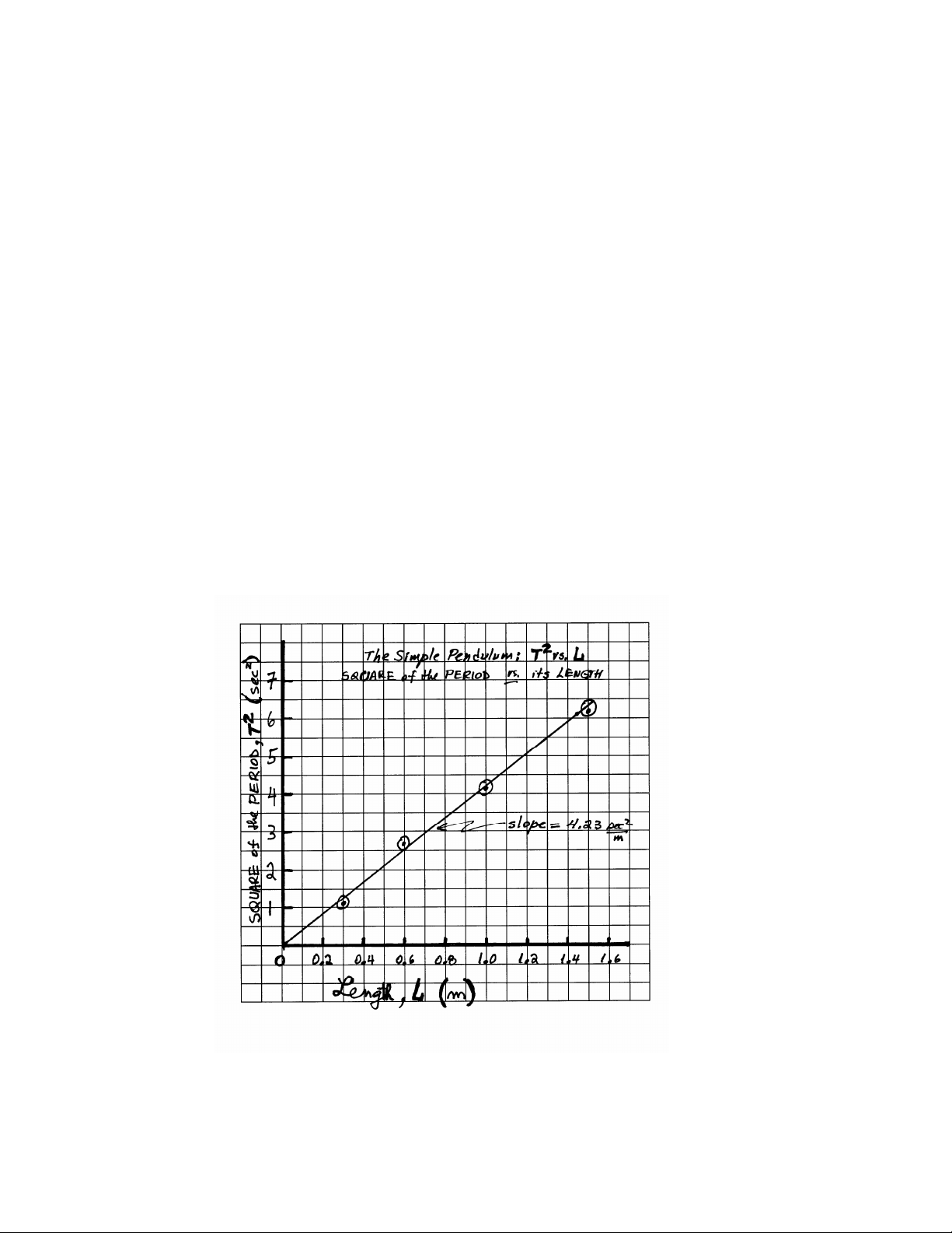
Start thinking about a nice title. For example, " The Square of the Period (T2) of a Simple Pendulum vs.
its Length (L)" [A shorter title would have been even better].
Keep your axes straight: If you need to plot "A vs B", or "A as a function of B", then A is on the vertical
axis and B is on the horizontal axis.
vertical axis = y-axis = the "ordinate"
horizontal axis = x-axis = the "abscissa"
The crucial part is choosing the range and scale for each axis. Two examples:
a) 0 to 5 sec; 5 graph boxes =1 sec.
b) -300 to +200 degrees; 2 boxes =100 degrees
The range must be just large enough to accommodate all your data and small enough that the scale is readable.
The scale should be spread out enough so your data take up most of the graph area, and labeled so
plotting (and reading) is easy.
Label the x and y-axis with the appropriate magnitudes. These should be round numbers which cover
the entire range of values that you will be plotting. A common mistake is to label too many boxes. If
you are trying to show that one quantity is proportional to another, or if you are not told otherwise, zero
is part of the range and must be located at the Origin. The numbers should be evenly spaced with the
same number of boxes between the same increase in numbers including the space from zero to the first
non-zero number. Choose an appropriate number of boxes between numbers. It is better to have 5
boxes between numbers than 4 since it is easier to interpolate in the first case than in the second.
(Similarly, 10 is better than 8, and 2 is better than 3.)
Plot the results of your measurements on this graph. Where appropriate, you should include error bars
to indicate the uncertainty in your measurements. These error bars are not of arbitrary size but should
be of the size of your uncertainty on the scale dictated by the numbers on the axis of your graph. 7
When you draw the line that best fits your data, the line should be a smooth one that need not go
through any points. In general, there should be as many points on one side of the line as on the other. If
you have done your work properly, the line should pass inside of the error bars for each point. (If it does
not, that may be an indication that there is something wrong with the point in question. Perhaps you
miss-recorded a measurement, or your estimate of the error was too small, or there was something wrong
with the apparatus, or with the technique you applied, etc.) If your graph shows that one quantity is
proportional to another, it should be a straight line that starts at the origin and passes through the plotted
data with as many points on one side as the other.
If you are asked to find the slope of the line, choose two points on the line that are as far apart as
possible. This will minimize the error that is introduced in reading the value of those points. The slope
is the difference between the vertical values of those points divided by the difference in the horizontal values of those points.
A common mistake is to measure the slope of the segment connecting two actual data points: this does
not yield the slope of the straight line you fitted to your data!
Note: Normally, the slope of your graphs has its own units, e.g., the slope of graph of velocity vs. time
has units of (m/s)/(s) = m/s2.
Here is a graph so messy, one can surely do better with a little practice. 8 LAB 1: DENSITY 1.1 INTRODUCTION
The MASS DENSITY of a body measures the amount of mass per unit volume of that body.
Definition: (Density of a body) = (body's mass)/(body's volume) or D = M / V
The density of a substance is independent of the shape or the particular amount of that substance.
For example, the density of a small gold ring and the density of a large gold brick should be the
same number, i.e., the density of gold.
In this lab you will measure the density of several different substances. As you do this, I hope you
will develop an appreciation for the concept of SIGNIFICANT FIGURES. You need to master the
concept of significant figures in order to succeed in this laboratory course.
As part of your density calculations you will need to compute the volume of a regular solid from its
linear dimensions. The quality of your volume measurements will thus depend on how precisely you can
measure lengths. You will use three progressively more precise instruments: a wooden “meter stick,”
vernier calipers, and a micrometer. Your instructor will demonstrate how to use each one. In each case,
read the instrument to the smallest division plus one more digit by estimation. So, a meter stick with
millimeter markings can be used to estimate a length to the nearest tenth of a millimeter, e.g., 12.4 mm,
or 1.24 cm. This estimate by “eye” is often good only to ±2 or 3, as you can verify by repeating the
measurement or asking your partner to do the estimating. A vernier is an invention that removes the
uncertainty in reading to the nearest tenth between adjacent markings, thus increasing the precision of
the final measurement. Your instructor will demonstrate how this is done with the vernier model,
prominently displayed in the front of the laboratory room.
On Errors and Uncertainty in a measurement:
When you work out a math computation, the numbers are usually considered exact, e.g., 1.1 x 1.2 x 1.3
= 1.716. But when a number represents a physical measurement it is never exact because of the
limitations of the instrument used, or the way it was employed, etc. It is essential, therefore, that each
experimental result be presented in a way that indicates its reliability. A very simple way to do this is by
the use of significant figures. (See Tutorial #1, on Significant Figures)
As an example, consider how different the following three cases are, even though they refer to exactly the same steel block:
a) 1.1 cm x 1.2 cm x 1.3 cm = 1.7 cm3
b) 1.13 cm x 1.20 cm x 1.29 cm = 1.75 cm3
c) 1.127 cm x 1.195 cm x 1.293 cm = 1.741 cm3
What is different about these three reports is the precision with which the data was measured. (By the 9
way, all three workers used significant figures correctly.)
Now, how accurate are the results? This concept reports on how close the reported answer is to the
"accepted answer". What determines accuracy? Examples are the calibration of the measuring
instruments or systematic errors on the part of whoever is taking the data. The following somewhat
oversimplified table may be useful in thinking about these concepts: Problem Remedy
____________________________________________________________________ Mistakes and blunders
Repeat measurements several times to check yourself Systematic errors
Use calibrated instruments properly and carefully Random errors
Treat data statistically and report on the average magnitude of errors 1.2 PRELAB ASSIGNMENT
After your lab instructor explains the concept of significant figures, complete the problems on the
page entitled, LAB 1: PRELAB ASSIGNMENT. Hand in your solutions before proceeding with the experiment. 1.3 PURPOSE
The objective of this laboratory exercise is to learn the concept of mass density and practice proper use
of significant figures. Another aim is to become familiar with instruments to measure length (meter
stick, vernier calipers, micrometer) and to appreciate the difference between accuracy and precision of experimental measurements.
1.4 EQUIPMENT AND SUPPLIES
Balance, metric ruler, wood blocks, metal blocks and cylinders, an aluminum block marked with
identifying letter, liquid samples and a graduated cylinder. 1.5 PROCEDURE!
Measuring the density of a block of maple wood.
Al. Familiarize yourself with the balance as you measure the mass of a maple wood block. Record the
mass of the block on the page labeled LAB 1: DATA SHEET.
A2. Measure the dimensions (length, width, thickness) of the maple wood block. Estimate to nearest
0.01cm by interpolating between millimeter markings. Record your data on the data sheet. 10
A3. Repeat the measurements carried out in A2 and record your data on the data sheet. Repeat
the measurements again and record. Do not forget units and the use of significant figures.
A4. Perform the computations required on the data sheet and obtain the best (or average)
dimensions, volume, density and percent deviation.
A5. Write your result for the density on the blackboard under the heading "Density of Maple
Wood" in a column of results provided by your classmates. Initial your own record.
Density of other solids.
Bl. You should be getting good by now at extracting maximum precision from the platform balance and
the metric scale. Follow the Data Sheet and make the necessary measurements in order to compute the
density of an aluminum block and cylinder. If time permits, continue with a brass block or cylinder and
an iron block. In each case, compute the percent deviation from the expected value.
B2. Attempt your most careful measurement on a block of aluminum. The aluminum block will be
marked with an identifying letter (A to Z). For this part of the lab exercise, do the work individually (without a partner). Density of liquids.
Cl. Obtain the density of water by the following procedure. Determine the mass of the DRY graduated
cylinder and record. Add about 50 cc (cubic cm) of tap water. Read and record the actual volume of
water in the graduated cylinder as precisely as you can, using the bottom of the meniscus as your
reference level. Obtain the combined mass of the graduated cylinder and water. From these data
compute the net mass of the water and, finally, the density of the water.
C2. Use the same procedure as in C1 to obtain the density of the colored alcohol solution that is
provided. CAUTION: Return all liquids to their proper containers.
DENSITY OF SOME SUBSTANCES (grams/cubic centimeter) aluminum 2.70 brass 8.90 water 1.00 lignum vitae 1.17 to 1.33 maple 0.62 to 0.68 balsa 0.12 to 0.20 iron 7.87 alcohol solution 0.80 lead 11.34 mercury 13.6 gold 19.3 11 12
LAB 2: ARCHIMEDES' PRINCIPLE INTRODUCTION
Archimedes' problem is said to have been the following: Determine (nondestructively!) if the king's new
gold crown contained within it baser metals. Whether or not the solution came to Archie in the bathtub,
the concepts of BUOYANCY and of SPECIFIC GRAVITY can provide the answer.
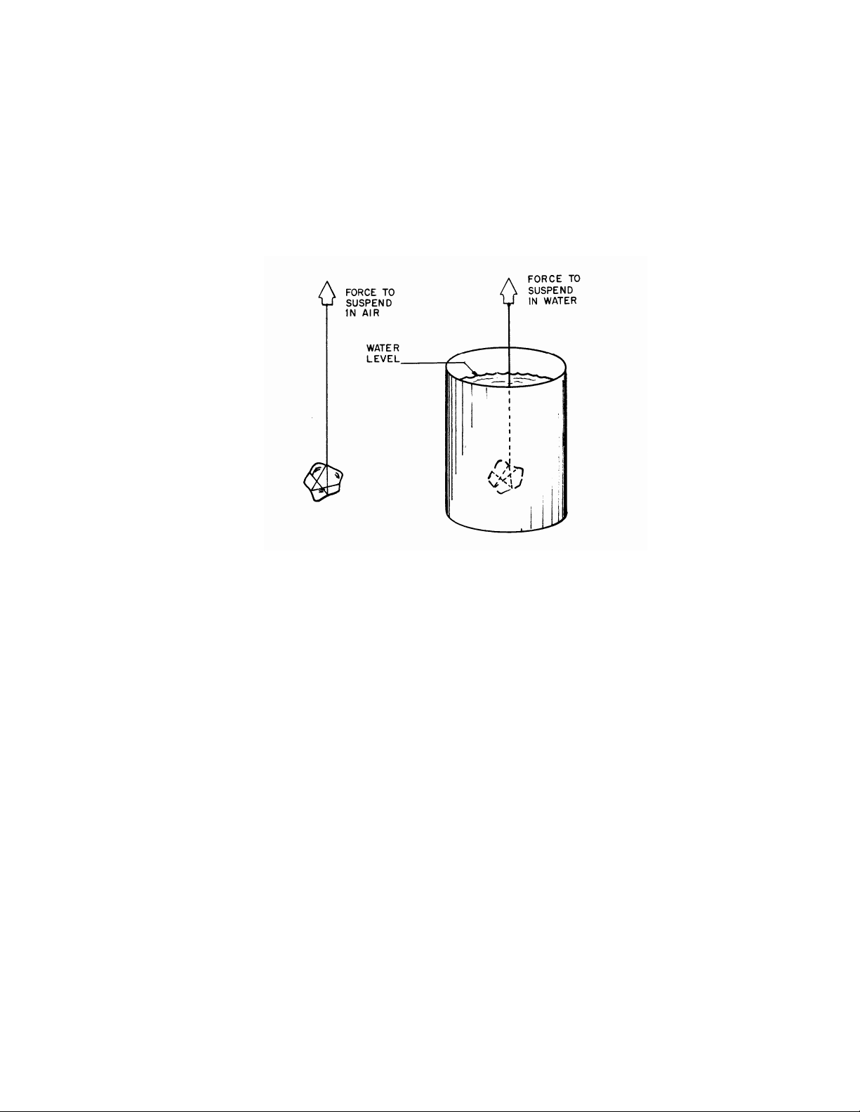
ARCHIMEDES' PRINCIPLE states that a body, partially or completely submerged in a fluid, is
buoyed up by a force equal to the weight of the fluid it displaces. The buoyant force B is then expressed
as the body's apparent loss of weight.
SPECIFIC GRAVITY is defined as the ratio of the density of a substance to the density of water.
An equivalent definition of this dimensionless quantity is: the ratio of the weight of a body to the
weight of an equal volume of water.
SPECIFIC GRAVITY of a chunk = Weight in air / Weight of water displaced
= Weight in air / Buoyant force
= Density of substance / Density of water
NOTE: The specific gravity of different substances is, in general, different. Thus, measuring the specific
gravity would help differentiate gold from lead. This was the brilliant idea that led Archimedes to shout "Eureka! " PURPOSE
The purpose of this experiment is to verify Archimedes' Principle and to determine the specific
gravity of certain substances. EQUIPMENT AND SUPPLIES
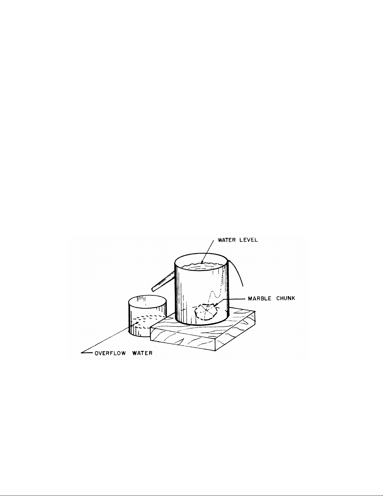
Test samples made of marble, metal and wood; balance, overflow can with spout, beaker, metal can,
1000 cc (cm3) graduated cylinder, metric ruler and some thread. 13 PROCEDURE
A. Measuring the specific gravity of an odd-shaped chunk of marble
Al. Measure and record the weight of a dry chunk of marble. If marble is wet, dry it with paper towels.
NOTE: To obtain the weight of an object in the proper units (i.e., units of force) simply multiply the
mass by g, the constant acceleration due to gravity (w=mg, where m represents mass and g is a constant equal to 9.8 m/s2).
A2. Measure the volume of the marble chunk by the following method. Fill the ‘overflow can with
spout’ so that an initial overflow runs out into the beaker. When the spout stops dripping, measure and
record the weight of the beaker containing the initial overflow water. Now, replace this same beaker and
gently lower the marble chunk into the overflow can. By doing so you will have collected the additional
water displaced by the chunk. The thread comes in handy in gently lowering the marble; if you had
thought of using your fingers, think again. Record the weight of the beaker with the additional overflow
water. Compute the net weight of water displaced by the chunk of marble. From the known density of
water, you can now compute the volume of the displaced water, and thus, the volume of the marble
chunk. Finally, compute the specific gravity of the marble chunk and record the result on the DATA SHEET.
Measuring the buoyant force on a submerged object 14
Bl. Pick a metal sample and record the weight and type of metal. Ask for help if you cannot distinguish
the various materials from each other.
B2. Determine the apparent weight of the metal when completely immersed in water. Do this by
suspending it with thread under the left-hand side of the platform balance, while it dangles fully immersed in the water can.
B3. Use paper towels to dry both the metal sample and your can. Now repeat procedure B2 using the
alcohol solution instead of water.
Specific gravity of a floating object (wood, in this case)
C1. Measure and record the weight and length of the block of wood.
C2. Fill the graduated cylinder with enough water so the block will float upright. Record the water level before immersing the block.
C3. Place the block upright in the cylinder and record the water level. You can now compute the volume
and the weight of water displaced by the block.
C4. Measure the average length of the part of the block remaining ABOVE the water level and
determine the length that is submerged.
C5. You can now compute the volume of the whole block using the following proportion: Total volume
divided by submerged volume equals the total length divided by the submerged length.
C6. What is the weight of water that has a volume equal to the volume of the block; i.e. how much water is displaced?
C7. The specific gravity of the wooden block is now just the ratio of its weight in air to the weight of an equal volume of water. 15 16
LAB 3: MOTION ON AN INCLINED PLANE INTRODUCTION
The distance d traveled by an object accelerating from rest is given by the expression d=1/2at2
where a is the acceleration and t is the time required for the object to travel a distance d starting from rest.
In this experiment you will measure the time it takes an object to roll 20, 40, 60, 80 and 100 cm for two
slightly different inclined plane angles. Each measurement of the time will enable you to compute a
value of the acceleration. Then, for each inclined plane, you will present all your data on a graph of d
versus the square of t. The equation above predicts that the points will fall on a straight line of slope (a/2).
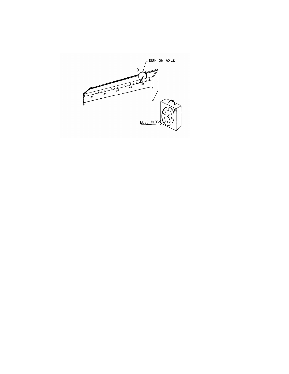
The apparatus provided is designed to generate small accelerations, so that the times for trips of a
distance of a meter or so are sufficiently long to be measured by a hand-operated clock. The effect of
gravity is decreased by using the inclined plane and by allowing the disks to roll on a thin axle. (This
trick was first realized by Galileo.) PURPOSE
The purpose of this laboratory exercise is to verify the constancy of acceleration of a disc rolling down
an inclined plane and to experimentally verify the equation displayed above. EQUIPMENT AND SUPPLIES
Inclined plane, disk mounted on axle, timer. 17 PROCEDURE
l. Using the inclined plane with both supports on the lab bench, make 3 determinations of the time
required for the disk to roll a distance of 20 cm starting from rest. Practice first until you can start the
disk in a repeatedly uniform fashion. Calculate the average time required for the three determinations,
the square of this time and the average acceleration. Make proper use of significant figures and record
your results on the data sheet provided.
2. Repeat for trips of 40 cm, 60 cm, 80 cm and 100 cm. Compute the average of the five values of
acceleration and the average of the percent deviations.
3. Increase the angle of inclination by letting the lower support of the plane extend over the edge of the
bench. Then repeat Procedures l and 2. 18