Planning as Heuristic Search
bai bao khoa hoc
Môn: Tài liệu Tổng hợp 3.6 K tài liệu
Trường: Tài liệu khác 3.9 K tài liệu
Tác giả:


Preview text:
Artificial Intelligence 129 (2001) 5–33 Planning as heuristic search
Blai Bonet ∗, Héctor Geffner
Depto. de Computación, Universidad Simón Bolívar, Aptdo. 89000, Caracas 1080-A, Venezuela Received 15 February 2000 Abstract
In the AIPS98 Planning Contest, the HSP planner showed that heuristic search planners can be
competitive with state-of-the-art Graphplan and SAT planners. Heuristic search planners like HSP
transform planning problems into problems of heuristic search by automatically extracting heuristics
from Strips encodings. They differ from specialized problem solvers such as those developed for the
24-Puzzle and Rubik’s Cube in that they use a general declarative language for stating problems and
a general mechanism for extracting heuristics from these representations.
In this paper, we study a family of heuristic search planners that are based on a simple and general
heuristic that assumes that action preconditions are independent. The heuristic is then used in the
context of best-first and hill-climbing search algorithms, and is tested over a large collection of
domains. We then consider variations and extensions such as reversing the direction of the search
for speeding node evaluation, and extracting information about propositional invariants for avoiding
dead-ends. We analyze the resulting planners, evaluate their performance, and explain when they
do best. We also compare the performance of these planners with two state-of-the-art planners, and
show that the simplest planner based on a pure best-first search yields the most solid performance
over a large set of problems. We also discuss the strengths and limitations of this approach, establish a
correspondence between heuristic search planning and Graphplan, and briefly survey recent ideas that
can reduce the current gap in performance between general heuristic search planners and specialized
solvers. 2001 Elsevier Science B.V. All rights reserved.
Keywords: Planning; Strips; Heuristic search; Domain-independent heuristics; Forward/backward search;
Non-optimal planning; Graphplan 1. Introduction
The last few years have seen a number of promising new approaches in Planning.
Most prominent among these are Graphplan [3] and Satplan [24]. Both work in stages * Corresponding author.
E-mail addresses: bonet@usb.ve (B. Bonet), hector@usb.ve (H. Geffner).
0004-3702/01/$ – see front matter 2001 Elsevier Science B.V. All rights reserved.
PII: S 0 0 0 4 - 3 7 0 2 ( 0 1 ) 0 0 1 0 8 - 4 6
B. Bonet, H. Geffner / Artificial Intelligence 129 (2001) 5–33
by building suitable structures and then searching them for solutions. In Graphplan,
the structure is a graph, while in Satplan, it is a set of clauses. Both planners have
shown impressive performance and have attracted a good deal of attention. Recent
implementations and significant extensions have been reported in [2,19,25,27].
In the recent AIPS98 Planning Competition [34], three out of the four planners in the
Strips track, IPP [19], STAN [27], and BLACKBOX [25], were based on these ideas. The
fourth planner, HSP [4], was based on the ideas of heuristic search [35,39]. In HSP, the
search is assumed to be similar to the search in problems like the 8-Puzzle, the main
difference being in the heuristic: while in problems like the 8-Puzzle the heuristic is
normally given (e.g., as the sum of Manhattan distances), in planning it has to be extracted
automatically from the declarative representation of the problem. HSP thus appeals to a
simple scheme for computing the heuristic from Strips encodings and uses the heuristic to guide the search for the goal.
The idea of extracting heuristics from declarative problem representations for guiding
the search in planning has been advanced recently by Drew McDermott [31,33], and by
Bonet, Loerincs and Geffner [6]. 1 In this paper, we extend these ideas, test them over
a large number of problems and domains, and introduce a family of planners that are
competitive with some of the best current planners.
Planners based on the ideas of heuristic search are related to specialized solvers such
as those developed for domains like the 24-Puzzle [26], Rubik’s Cube [23], and Sokoban
[17] but differ from them mainly in the use of a general language for stating problems and
a general mechanism for extracting heuristics. Heuristic search planners, like all planners,
are general problem solvers in which the same code must be able to process problems from
different domains [37]. This generality comes normally at a price: as noted in [17], the
performance of the best current planners is still well behind the performance of specialized
solvers. Closing this gap, however, is the main challenge in planning research where the
ultimate goal is to have systems that combine flexibility and efficiency: flexibility for
modeling a wide range of problems, and efficiency for obtaining good solutions fast. 2
In heuristic search planning, this challenge can only be met by the formulation, analysis,
and evaluation of suitable domain-independent heuristics and optimizations. In this paper
we aim to present the basic ideas and results we have obtained, and discuss more recent
ideas that we find promising. 3
More precisely, we will present a family of heuristic search planners based on a simple
and general heuristic that assumes that action preconditions are independent. This heuristic
is then used in the context of best-first and hill-climbing search algorithms, and is tested
over a large class of domains. We also consider variations and extensions, such as reversing
the direction of the search for speeding node evaluation, and extracting information about
propositional invariants for avoiding dead-ends. We compare the resulting planners with
1 This idea also appears, in a different form, in the planner IxTex; see [29].
2 Interestingly, the area of constraint programming has similar goals although it is focused on a different class
of problems [16]. Yet, see [45] for a recent attempt to apply the ideas of constraint programming in planning.
3 Another way to reduce the gap between planners and specialized solvers is by making room in planning
languages for expressing domain-dependent control knowledge (e.g., [5]). In this paper, however, we don’t
consider this option which is perfectly compatible and complementary with the ideas that we discuss.
B. Bonet, H. Geffner / Artificial Intelligence 129 (2001) 5–33 7
some of the best current planners and show that the simplest planner based on a pure best-
first search, yields the most solid performance over a large set of problems. We also discuss
the strengths and limitations of this approach, establish a correspondence between heuristic
search planning and Graphplan, and briefly survey recent ideas that can help reduce the
performance gap between general heuristic search planners and specialized solvers.
Our focus is on non-optimal sequential planning. This is contrast with the recent
emphasis on optimal parallel planning following Graphplan and SAT-based planners [24].
Algorithms are evaluated in terms of the problems that they solve (given limited time and
memory resources), and the quality of the solutions found (measured by the solution time
and length). The use of heuristics for optimal sequential and parallel planning is considered
in [13] and is briefly discussed in Section 8.
In this paper we review and extend the ideas and results reported in [4]. However, rather
than focusing on the two specific planners HSP and HSPr, we consider and analyze a
broader space of alternatives and perform a more exhaustive empirical evaluation. This
more systematic study led us to revise some of the conjectures in [4] and to understand
better the strengths and limitations involved in the choice of the heuristics, the search
algorithms, and the direction of the search.
The rest of the paper is organized as follows. We cover first general state models
(Section 2) and the state models underlying problems expressed in Strips (Section 3). We
then present a domain-independent heuristic that can be obtained from Strips encodings
(Section 4), and use this heuristic in the context of forward and backward state planners
(Sections 5 and 6). We then consider related work (Section 7), summarize the main ideas
and results, and discuss current open problems (Section 8). 2. State models
State spaces provide the basic action model for problems involving deterministic actions
and complete information. A state space consists of a finite set of states S, a finite set
of actions A, a state transition function f that describes how actions map one state into
another, and a cost function c(a, s) > 0 that measures the cost of doing action a in state
s [35,38]. A state space extended with a given initial state s0 and a set SG of goal states
will be called a state model. State models are thus the models underlying most of the
problems considered in heuristic search [39] as well as the problems that fall into the scope
of classical planning [35]. Formally, a state model is a tuple S = S, s0, SG, A, f, c where
• S is a finite and non-empty set of states s,
• s0 ∈ S is the initial state,
• SG ⊆ S is a non-empty set of goal states,
• A(s) ⊆ A denotes the actions applicable in each state s ∈ S,
• f (a, s) denotes a state transition function for all s ∈ S and a ∈ A(s), and
• c(a, s) stands for the cost of doing action a in state s.
A solution of a state model is a sequence of actions a0, a1, . . . , an that generates a state
trajectory s0, s1 = f (s0), . . . , sn+1 = f (an, sn) such that each action ai is applicable in si
and sn+1 is a goal state, i.e., ai ∈ A(si) and sn+1 ∈ SG. The solution is optimal when the total cost n c(a i=0 i , si ) is minimized. 8
B. Bonet, H. Geffner / Artificial Intelligence 129 (2001) 5–33
In problem solving, it is common to build state models adapted to the target domain
by explicitly defining the state space and explicitly coding the state transition function
f (a, s) and the action applicability conditions A(s) in a suitable programming language.
In planning, state models are defined implicitly in a general declarative language that
can easily accommodate representations of different problems. We consider next the state
models underlying problems expressed in the Strips language [9]. 4
3. The Strips state model
A planning problem in Strips is represented by a tuple P = A, O, I, G where A is
a set of atoms, O is a set of operators, and I ⊆ A and G ⊆ A encode the initial and goal
situations. The operators op ∈ O are all assumed grounded (i.e., with the variables replaced
by constants). Each operator has a precondition, add, and delete lists denoted as Prec(op),
Add(op), and Del(op) respectively. They are all given by sets of atoms from A. A Strips
problem P = A, O, I, G defines a state space SP = S, s0, SG, A(·), f, c where
(S1) the states s ∈ S are collections of atoms from A;
(S2) the initial state s0 is I ;
(S3) the goal states s ∈ SG are such that G ⊆ s;
(S4) the actions a ∈ A(s) are the operators op ∈ O such that Prec(op) ⊆ s;
(S5) the transition function f maps states s into states s = s − Del(a) + Add(a) for a ∈ A(s);
(S6) all action costs c(a, s) are 1.
The (optimal) solutions of the problem P are the (optimal) solutions of the state model
SP . A possible way to find such solutions is by performing a search in such space. This
approach, however, has not been popular in planning where approaches based on divide-
and-conquer ideas and search in the space of plans have been more common [35,46].
This situation however has changed in the last few years, after Graphplan [3] and SAT
approaches [24] achieved orders of magnitude speed ups over previous approaches. More
recently, the idea of planning as state space search has been advanced in [31] and [6]. In
both cases, the key ingredient is the heuristic used to guide the search that is extracted
automatically from the problem representation. Here we follow the formulation in [6]. 4. Heuristics
The heuristic function h for solving a problem P in [6] is obtained by considering a
‘relaxed’ problem P in which all delete lists are ignored. From any state s, the optimal
cost h(s) for solving the relaxed problem P can be shown to be a lower bound on the
optimal cost h∗(s) for solving the original problem P . As a result, the function h(s) could
be used as an admissible heuristic for solving the original problem P . However, solving the
‘relaxed’ problem P and obtaining the function h are NP-hard problems. 5 We thus use an
4 As it is common, we use the current version of the Strips language as defined by the Strips subset of PDDL
[32] rather than original version in [9].
5 This can be shown by reducing set-covering to Strips with no deletes.
B. Bonet, H. Geffner / Artificial Intelligence 129 (2001) 5–33 9
approximation and set h(s) to an estimate of the optimal value function h(s) of the relaxed
problem. In this approximation, we estimate the cost of achieving the goal atoms from s
and then set h(s) to a suitable combination of those estimates. The cost of individual atoms
is computed by a procedure which is similar to the ones used for computing shortest paths
in graphs [1]. Indeed, the initial state and the actions can be understood as defining a graph
in atom space in which for every action op there is a directed link from the preconditions
of op to its positive effects. The cost of achieving an atom p is then reflected in the length
of the paths that lead to p from the initial state. This intuition is formalized below.
We will denote the cost of achieving an atom p from the state s as gs(p). These estimates
can be defined recursively as 6 0 if p ∈ s, gs (p) =
min [1 + gs(Prec(op))] otherwise, (1) op∈O(p)
where O(p) stands for the actions op that add p, i.e., with p ∈ Add(op), and gs(Prec(op)),
to be defined below, stands for the estimated cost of achieving the preconditions of action op from s.
While there are many algorithms for obtaining the function gs defined by (1), we use
a simple forward chaining procedure in which the measures gs(p) are initialized to 0 if
p ∈ s and to ∞ otherwise. Then, every time an operator op is applicable in s, each atom
p ∈ Add(op) is added to s and gs(p) is updated to
gs (p) := min gs(p), 1 + gs Prec(op) . (2)
These updates continue until the measures gs (p) do not change. It’s simple to show that
the resulting measures satisfy Eq. (1). The procedure is polynomial in the number of atoms
and actions, and corresponds essentially to a version of the Bellman–Ford algorithm for
finding shortest paths in graphs [1].
The expression gs(Prec(op)) in both (1) and (2) stands for the estimated cost of the set
of atoms given by the preconditions of action op. In planners such as HSP, the cost gs (C) of
a set of atoms C is defined in terms of the cost of the atoms in the set. As we will see below,
this can be done in different ways. In any case, the resulting heuristic h(s) that estimates
the cost of achieving the goal G from a state s is defined as def h(s) = gs(G). (3)
The cost gs (C) of sets of atoms can be defined as the weighted sum of costs of individual
atoms, the minimum of the costs, the maximum of the costs, etc. We consider two ways.
The first is as the sum of the costs of the individual atoms in C: g+ s (C) = gs (r) (additive costs). (4) r∈C
We call the heuristic that results from setting the costs gs (C) to g+
s (C), the additive
heuristic and denote it by hadd. The heuristic hadd assumes that subgoals are independent.
This is not true in general as the achievement of some subgoals can make the achievement
6 Where the min of an empty set is defined to be infinite. 10
B. Bonet, H. Geffner / Artificial Intelligence 129 (2001) 5–33
of the other subgoals more or less difficult. For this reason, the additive heuristic is not
admissible (i.e., it may overestimate the true costs). Still, we will see that it is quite useful in planning.
Second, an admissible heuristic can be defined by combining the cost of atoms by the max operation as: gmax s
(C) = max gs(r) (max costs). (5) r∈C
We call the heuristic that results from setting the costs gs (C) to gmax s
(C), the max heuristic
and denote it by hmax. The max heuristic unlike the additive heuristic is admissible as the
cost of achieving a set of atoms cannot be lower than the cost of achieving each of the
atoms in the set. On the other hand, the max heuristic is often less informative. In fact,
while the additive heuristic combines the costs of all subgoals, the max heuristic focuses
only on the most difficult subgoals ignoring all others. In Section 7, however, we will see
that a refined version of the max heuristic is used in Graphplan.
5. Forward state planning
5.1. HSP: A hill-climbing planner
The planner HSP [4] that was entered into the AIPS98 Planning Contest, uses the additive
heuristic hadd to guide a hill-climbing search from the initial state to the goal. The hill-
climbing search is very simple: at every step, one of the best children is selected for
expansion and the same process is repeated until the goal is reached. Ties are broken
randomly. The best children of a node are the ones that minimize the heuristic hadd. Thus,
in every step, the estimated atom costs gs(p) and the heuristic h(s) are computed for the
states s that are generated. In HSP, the hill climbing search is extended in several ways; in
particular, the number of consecutive plateau moves in which the value of the heuristic hadd
is not decremented is counted and the search is terminated and restarted when this number
exceeds a given threshold. In addition, all states that have been generated are stored in a
fast memory (a hash table) so that states that have been already visited are avoided in the
search and their heuristic values do not have to be recomputed. Also, a simple scheme for
restarting the search from different states is used for avoiding getting trapped into the same plateaus.
Many of the design choices in HSP are ad-hoc. They were motivated by the goal of
getting a better performance for the Planning Contest and by our earlier work on a real-
time planner based on the same heuristic [6]. HSP did well in the Contest competing in the
“Strips track” against three state-of-the-art Graphplan and SAT planners: IPP [19], STAN
[27] and BLACKBOX [25]. Table 1 from [34] shows a summary of the results. In the contest
there were two rounds with 140 and 15 problems each, in both cases drawn from several
domains. The table shows for each planner in each round, the number of problems solved,
the average time taken over the problems that were solved, and the number of problems in
which each planner was fastest or produced shortest solutions. IPP, STAN and BLACKBOX,
are optimal parallel planners that minimize the number of time steps (in which several
actions can be performed concurrently) but not the number of actions.
B. Bonet, H. Geffner / Artificial Intelligence 129 (2001) 5–33 11 Table 1
Results of the AIPS98 Contest (Strips track). Columns show the number of problems
solved by each planner, the average time over the problems solved (in seconds) and
the number of problems in which each planner was fastest or produced shortest plans (from [34]) Round Planner Avg. time Solved Fastest Shortest Round 1 BLACKBOX 1.49 63 16 55 HSP 35.48 82 19 61 IPP 7.40 63 29 49 STAN 55.41 64 24 47 Round 2 BLACKBOX 2.46 8 3 6 HSP 25.87 9 1 5 IPP 17.37 11 3 8 STAN 1.33 7 5 4
As it can be seen from the table, HSP solved more problems than the other planners but
it often took more time or produced longer plans. More details about the setting and results
of the competition can be found in [34] and in an article to appear in the AI Magazine.
5.2. HSP2: A best-first search planner
The results above and a number of additional experiments suggest that HSP is
competitive with the best current planners over many domains. However, HSP is not an
optimal planner, and what’s worse—considering that optimality has not been a traditional
concern in planning—the search algorithm in HSP is not complete. In this section, we
show that this last problem can be overcome by switching from hill-climbing to a best-first
search (BFS) [39]. Moreover, the resulting BFS planner is superior in performance to HSP,
and it appears to be superior to some of the best planners over a large class of problems.
By performance we mean: the number of problems solved, the time to get those solutions,
and the length of those solutions measured by the number of actions.
We will refer to the planner that results from the use of the additive heuristic hadd in a
best-first search from the initial state to the goal, as HSP2. This best-first search keeps an
Open and a Closed list of nodes as ∗ A
[35,39] but weights nodes by an evaluation function
f (n) = g(n) + W · h(n), where g(n) is the accumulated cost, h(n) is the estimated cost
to the goal, and W 1 is a constant. For W = 1, the algorithm is ∗ A and for W = 1 it corresponds to the so-called ∗ WA
algorithm [39]. Higher values of W usually lead to the
goal faster but with solutions of lower quality [22]. Indeed, if the heuristic is admissible, the solutions found by ∗ WA
are guaranteed not to exceed the optimal costs by more than a factor of W . ∗
HSP2 uses the WA algorithm with the non-admissible heuristic hadd which is
evaluated from scratch in every new state generated. The value of the parameter W is fixed
at 5, even though values in the range [2, 10] do not make a significant difference. 12
B. Bonet, H. Geffner / Artificial Intelligence 129 (2001) 5–33 5.3. Experiments
In the experiments below, we assess the performance of the two heuristic search
planners, HSP and HSP2, in comparison with two state-of-the-art planners, STAN 3.0 [27],
and BLACKBOX 3.6 [25]. HSP and HSP2 both perform a forward state space search guided
by the additive heuristic hadd. The first performs an extended hill-climbing search and
the later performs a best-first search with an evaluation function in which the heuristic is
multiplied by the constant W = 5. STAN and BLACKBOX are both based on Graphplan [3],
but the latter maps the plan graph into a set of clauses that are checked for satisfiability.
The version of HSP used in the experiments, HSP 1.2, improves the version used in the
AIPS98 Contest and the one used in [4].
For each planner and each planning problem we evaluate whether the planner solves
the problem, and if so, the time taken by the planner and the number of actions in the
solution. STAN and BLACKBOX are optimal parallel planners that minimize the number of
time steps but not necessarily the number of actions. Both planners were run with their default options.
The experiments were performed on an Ultra-5 with 128 Mb RAM and 2 Mb of Cache
running Solaris 7 at 333 MHz. The exception are the results for BLACKBOX on the
Logistics problems that were taken from the BLACKBOX distribution as the default options
produced much poorer results. 7 The domains considered are: Blocks, Logistics, Gripper,
8-Puzzle, Hanoi, and Tire-World. They constitute a representative sample of difficult but
solvable instances for current planners. Five of the 10 Blocks-World instances are of our
own [4], the rest of the problems are taken from others as noted. A planner is said not
to solve a problem when it either runs out of memory or runs out of time (10 minutes).
Failure to find solutions due either to memory or time constraints are displayed as plans with length −1.
All the planners are implemented in C and accept problems in the PDDL language (the
standard language used in the AIPS98 Contest; [32]). Moreover, the planners in the HSP
family convert every problem instance in PDDL into a program in C. Generating, compiling,
linking, and loading such program takes in the order of 2 seconds. This time is roughly
constant for all instances and domains, and is not included in the figures below. 5.3.1. Blocks-World
The first experiments deal with the blocks world. The blocks world is challenging
for domain-independent planners due to the interactions among subgoals and the size of
the state space. The ten instances considered involve from 7 to 19 blocks. Five of these
instances are taken from the BLACKBOX distribution and five are from [4]. The results for
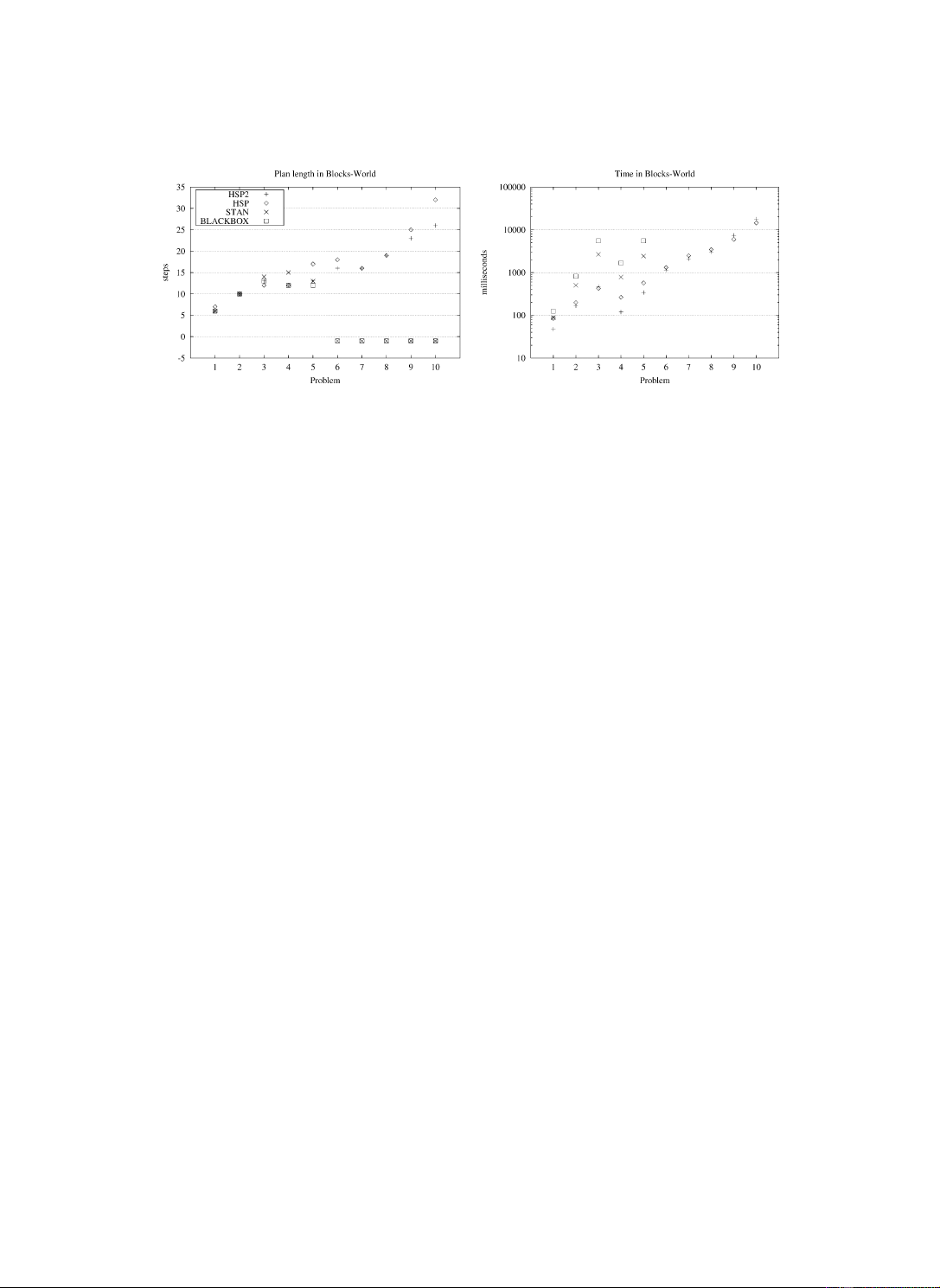
this domain are shown in Fig. 1 that displays for each planner the length of the solutions
on the left, and the time to get those solutions on the right.
The lengths produced by STAN and BLACKBOX are not necessarily optimal in this
domain as there is some parallelism (e.g., moving blocks among disjoint pairs of towers).
This is the reason the lengths they report do not always coincide. In any case, the solutions
reported by the four planners are roughly equivalent over instances 1–5, with STAN and HSP
7 Those results were obtained on a SPARC Ultra 2 with a 296 MHz clock and 256 M of RAM [5].
B. Bonet, H. Geffner / Artificial Intelligence 129 (2001) 5–33 13
Fig. 1. Solution length (left) and time (right) over 10 Blocks-World instances.
producing slightly longer solutions for instances 4 and 5. Over the more difficult instances
6–10, the situation changes and only HSP and HSP2 report solutions, with the plans found
by HSP2 being shorter. Regarding solution times, the times for HSP and HSP2 are roughly
even, and slightly shorter than those for STAN and BLACKBOX over the first five instances.
Over the last five instances STAN and BLACKBOX run out of memory. 5.3.2. Logistics
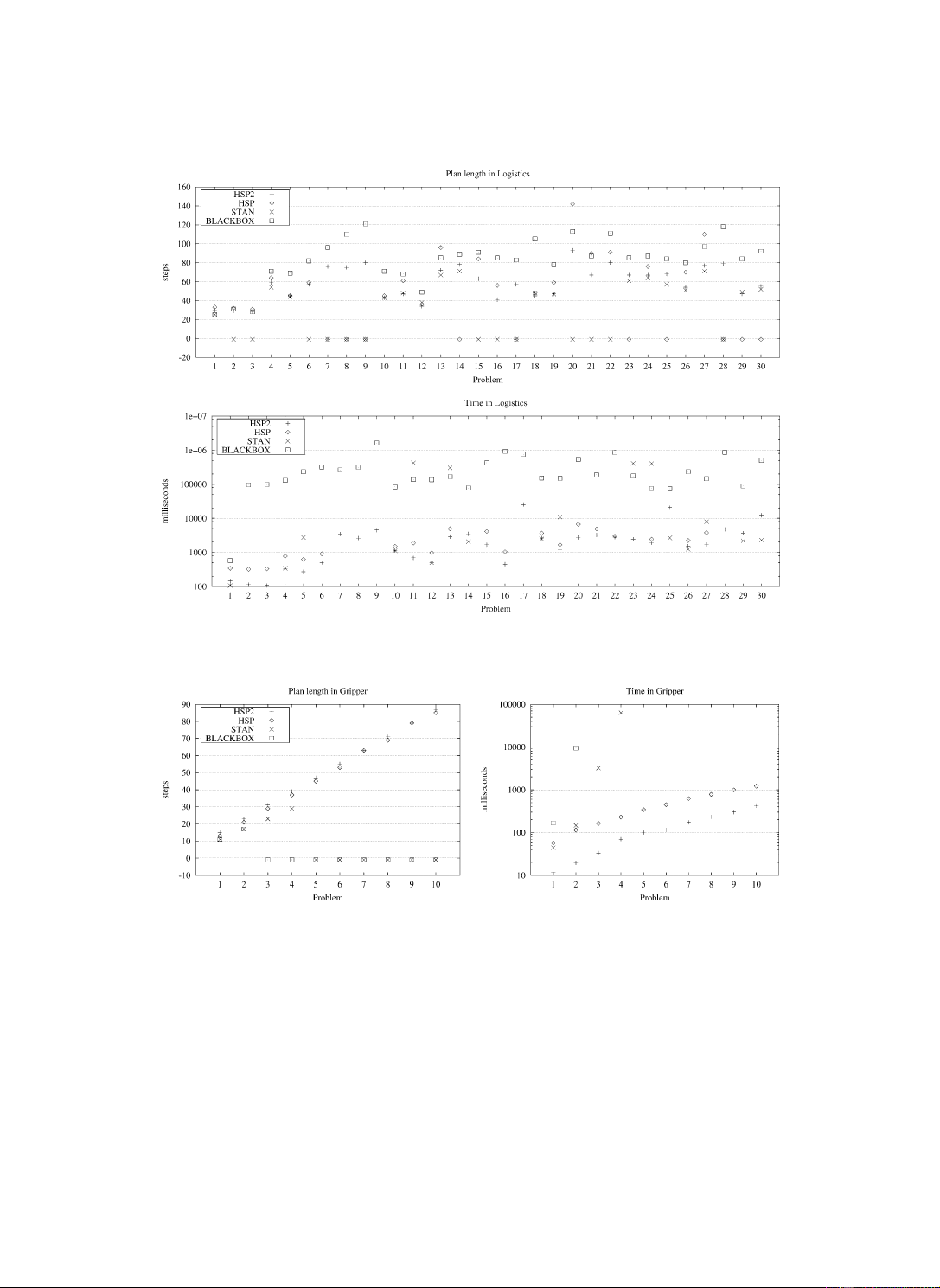
The second set of experiments deals with the logistics domain, a domain that involves
the transportation of packages by either trucks or airplanes. Trucks can move among
locations in the same city, and airplanes can move between airports in one city to airports
in another city. Packages can be loaded and unloaded in trucks and airplanes, and the task
is to transport them from their original locations to some target locations. This is a highly
parallel domain, where many operations can be done in parallel. As a result, plans involve
many actions but the number of time steps is usually much smaller. The domain is from
Kautz and Selman from an earlier version due to Manuela Veloso. The 30 instances we
consider are from the BLACKBOX distribution.
The results for this domain are shown in Fig. 2. The number of actions in the plans are
reported on the upper plot, times are reported on the lower plot, and failures to find a plan
are reported with length −1. Both HSP2 and BLACKBOX solve all 30 instances, HSP2 being
roughly two orders of magnitude faster. STAN and HSP, on the other hand, fail on 13 and 10
instances respectively. Interestingly, the times reported by STAN on the instances it solves
tend to be close to those reported by HSP2. On the other instances STAN runs out of memory
(instances 3, 16, 17, 20, 22, 28) or time (instances 2, 6, 7, 8, 9, 15, 21). 5.3.3. Gripper
The third set of experiments deals with the Gripper domain used in the AIPS98 Planning
Contest and due to J. Koehler. This is a domain that concerns a robot with two grippers
that must transport a set of balls from one room to another. It is very simple for humans
to solve but in the Planning Contest proved difficult to most of the planners. Indeed, the
domain is not challenging for specialized solvers, but is challenging for certain types of domain-independent planners. 14
B. Bonet, H. Geffner / Artificial Intelligence 129 (2001) 5–33
Fig. 2. Solution length (upper) and time (lower) over 30 Logistics instances from Kautz and Selman.
Fig. 3. Solution length (left) and time (right) over 10 Gripper instances from AIPS98 Contest.
The results over 10 Gripper instances from the AIPS98 Contest are shown in Fig. 3.
The planners HSP and HSP2 have no difficulties and compute plans with similar lengths.
On the other hand, BLACKBOX solves the first two instances only, and STAN the first four
instances. As shown on the right, the time required by both planners grows exponentially
and they run out of time over the larger instances. On the other hand, HSP and HSP2 scale
up smoothly with HSP2 being slightly faster than HSP.
B. Bonet, H. Geffner / Artificial Intelligence 129 (2001) 5–33 15
One of the reasons for the failure of both STAN and BLACKBOX in Gripper is that the
heuristic implicitly represented by the plan graph is a very poor estimator in this domain.
As a result, Graphplan-based planners, such as STAN and BLACKBOX that perform a form of ∗ IDA
search must do many iterations before finding a solution. Actually, the same
exponential growth in Gripper occurs also in HSP planners when the heuristic hmax is used
in place of the additive heuristic. As before, the problem is that the hmax heuristic is almost
useless in this domain where subgoals are mostly independent. The heuristic implicit in
the plan graph is a refinement of the hmax heuristic; the relation between Graphplan and
heuristic search planning will be analyzed further in Section 7. 5.3.4. Puzzle
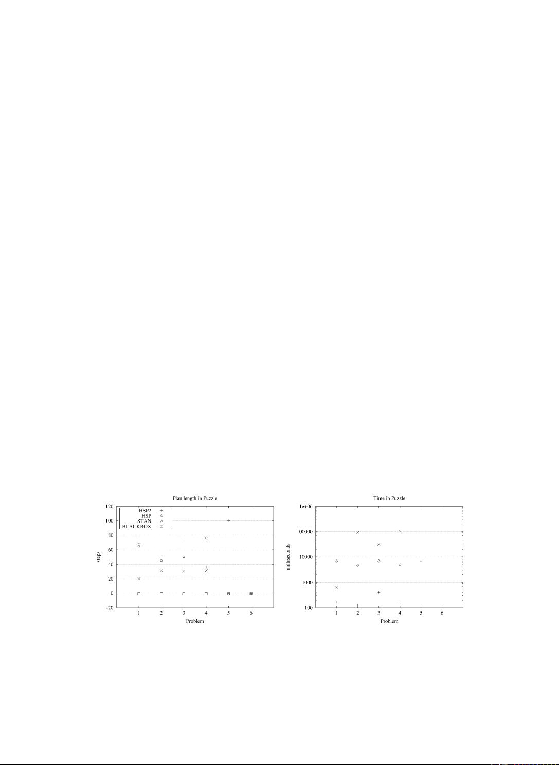
The next problems are four instances of the familiar 8-Puzzle and two instances from the
larger 15-Puzzle. Three of the four 8-Puzzle instances are hard as their optimal solutions
involves 31 steps, the maximum plan length in such domain. The 15-Puzzle instances are of medium difficulty.
As shown in Fig. 4, HSP and STAN solve the first four instances, and HSP2 solves the first
five. The solutions computed by STAN are optimal in this domain which is purely serial.
The solutions computed by HSP and HSP2, on the other hand, are poorer, and are often twice
as long. On the other hand, as shown on the left part of the figure, HSP2 is two orders of
magnitude faster than STAN over the difficult 8-Puzzle instances (2–4) and can also solve
instance 5. The times for HSP are worse and does not solve instance 5. BLACKBOX does
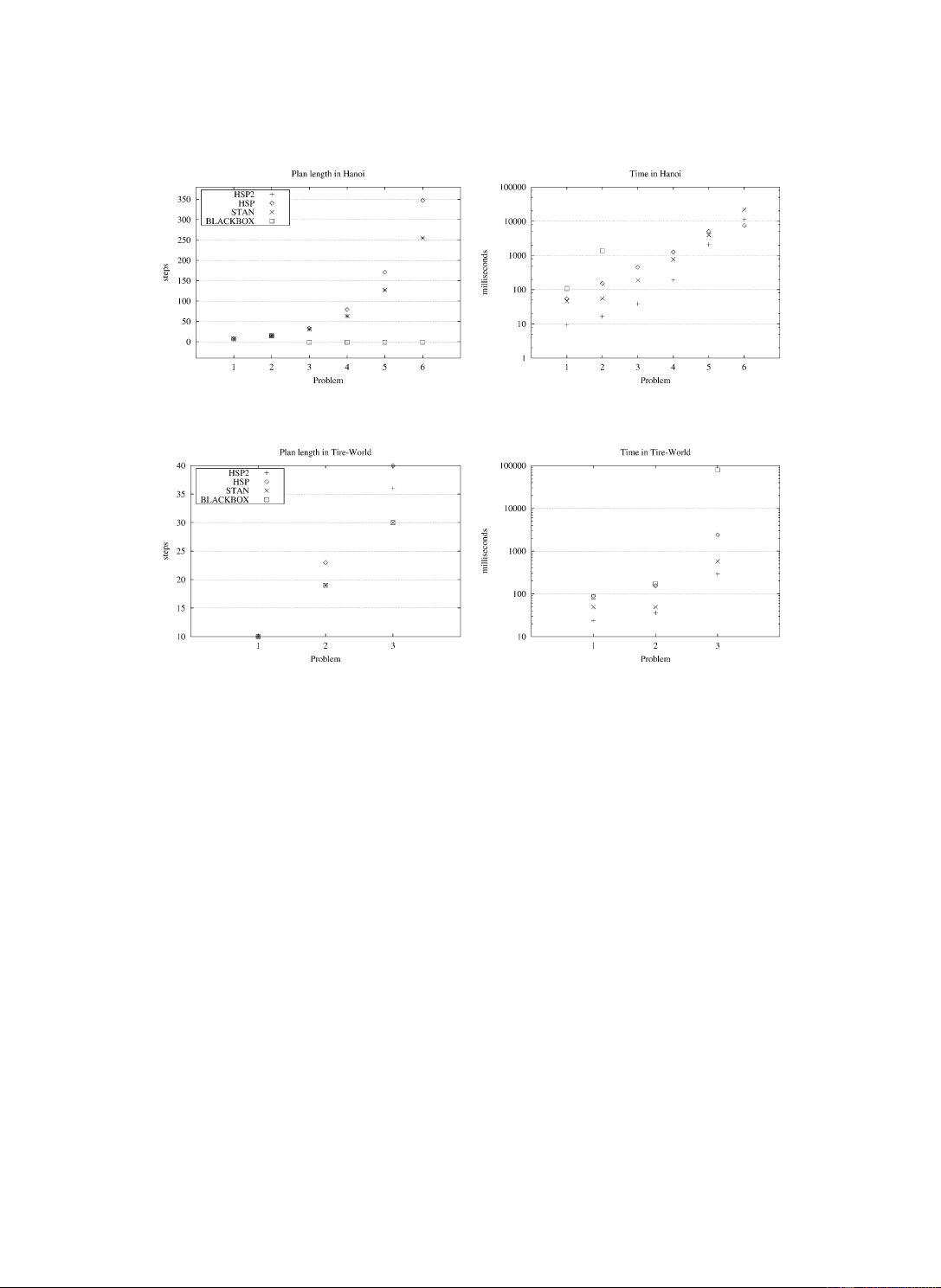
not solve any of the instances. 5.3.5. Hanoi
Fig. 5 shows the results for Hanoi. Instance i has i + 2 disks, thus problems range from
3 disks up to 8 disks. Over all these problems HSP2 and STAN generate plans of the same
quality, HSP2 being slightly faster than STAN. HSP also solves all instances but the solutions
are longer. BLACKBOX solves the first two instances.
Fig. 4. Solution length (left) and time (right) over four instances of the 8-Puzzle (1–4) and two instances of the 15-Puzzle (5–6). 16
B. Bonet, H. Geffner / Artificial Intelligence 129 (2001) 5–33
Fig. 5. Solution length (left) and time (right) over six Hanoi instances. Instance i has i + 2 disks.
Fig. 6. Solution length (left) and time (right) over three instances of Tire-World. 5.3.6. Tire-World
The Tire-World domain is due to S. Russell and involves operations for fixing flat tires:
opening and closing the trunk of a car, fetching and putting away tools, loosening and
tightening nuts, etc. Fig. 6 shows the results. Here both STAN and BLACKBOX solve all
three instances producing optimal plans. HSP and HSP2 also solve these instances but in
some cases they produce inferior solutions. On the time scale, HSP2 is slightly faster than
STAN, and both are faster than BLACKBOX in one case by two orders of magnitude. As
before, HSP is slower than HSP2 and produces longer solutions.
5.4. Summary: Forward state planning
The experiments above, based on a representative sample of problems, show that the two
forward heuristic search planners HSP and HSP2 are capable of solving the problems solved
by two state-of-the-art planners. In addition, in some domains, HSP and in particular HSP2
solve problems that the other planners with their default settings do not currently solve.
The planner HSP2, based on a standard best first search, tends to be faster and more robust
than the hill-climbing HSP planner. Thus, the arguments in [4] in support of a hill-climbing
strategy based on the slow node generation rate that results from the computation of the
B. Bonet, H. Geffner / Artificial Intelligence 129 (2001) 5–33 17
heuristic in every state do not appear to hold in general. Indeed, the combination of the
additive heuristic hadd and the multiplying constant W > 1 often drive the best-first planner
to the goal with as few node evaluations as the hill-climbing planner, already providing the
necessary ‘greedy’ bias. An ∗ A
search with an admissible and consistent heuristic, on the
other hand, is bound to expand all nodes n whose cost f (n) is below the optimal cost. This however does no apply to the ∗ WA strategy used in HSP2.
In the experiments the W parameter in HSP2 was set to the constant value 5. Yet HSP2 is
not particularly sensitive to the exact value of this constant. Indeed, in most of the domains,
values in the interval [2, 10] produce similar results. This is likely due to the fact that the
heuristic hadd is not admissible and by itself tends to overestimate the true costs without
the need of a multiplying factor. On the other hand, in some domains like Logistics and
Gripper, the value W = 1 does not lead to solutions. This is precisely because in these
domains that involve subgoals that are mostly independent, the additive heuristic is not
‘sufficiently’ overestimating. Finally, in problems like the sliding tile puzzles, values of
W closer to 1 produce better solutions in more time, in correspondence with the normal
pattern observed in cases in which the heuristic is admissible [22].
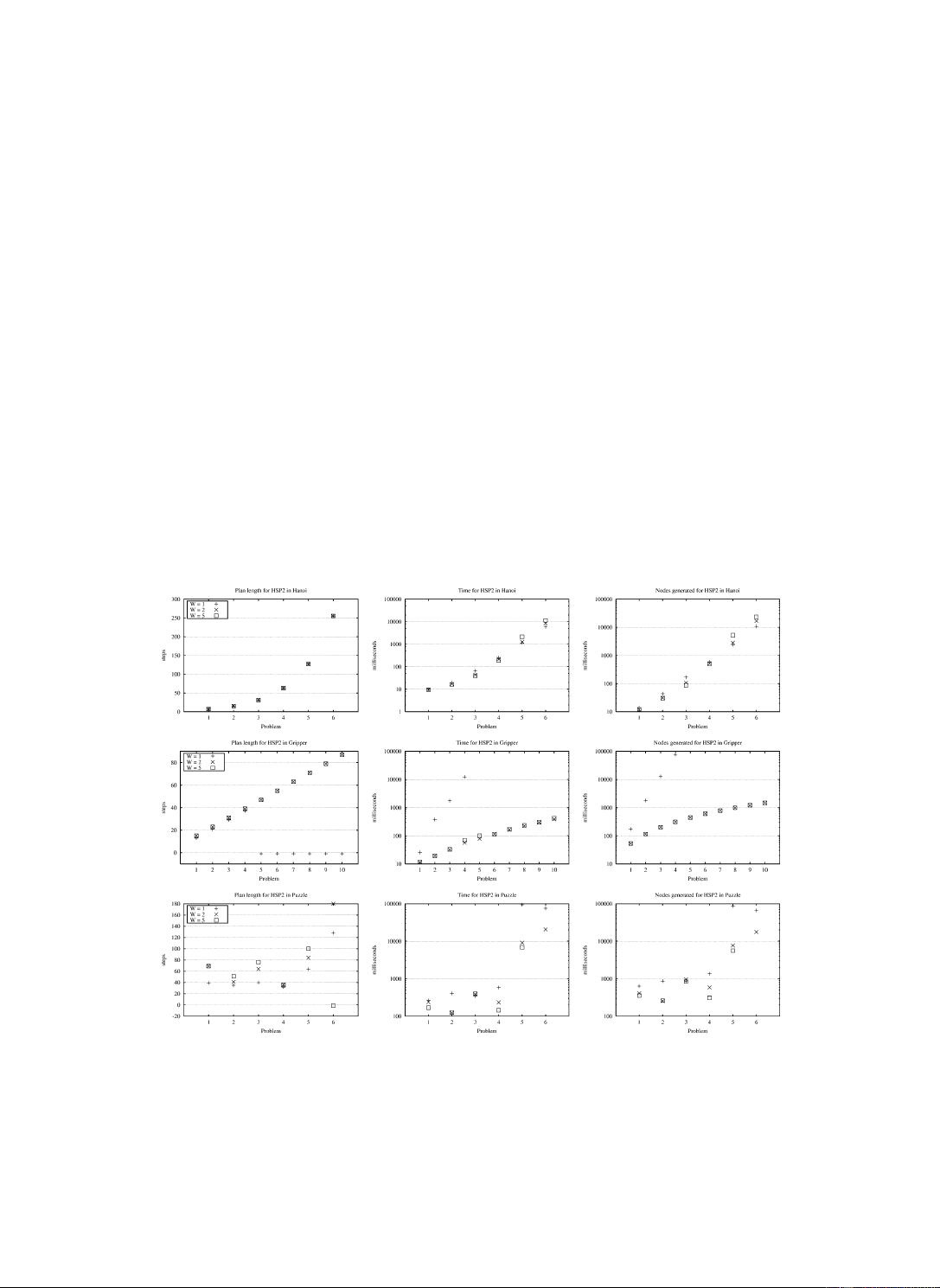
Fig. 7 shows the effects of three different values of W on the quality and times of the
solutions, and the number of nodes generated. The values considered are W = 1, W = 2,
and W = 5. The top three curves that correspond to Hanoi, are typical for most of the other
Fig. 7. Influence of value of W in the HSP2 planner on the length of the solutions (left), the time required to find
solutions (center), and number of nodes generated (right). The domains from top to bottom are Hanoi, Gripper, and Puzzle. 18
B. Bonet, H. Geffner / Artificial Intelligence 129 (2001) 5–33
domains and show little effect. The second set of curves corresponds to Gripper where
HSP2 fails to solve the last six instances for W = 1. Indeed, the two right most curves show
an exponential growth in time and the number of generated nodes. In Logistics, HSP2 with
W = 1 also fails to solve most of the instances. As noted above, these are two domains
where subgoals are mostly independent and where the additive heuristic is not sufficiently
overestimating and hence fails to provide the ‘greedy bias’ necessary to find the solutions.
Indeed, the state space in Logistics is very large, while in Gripper it’s the branching factor
that is large due to the (undetected) symmetries in the problem.
The bottom set of curves in Fig. 7 correspond to the Puzzle domain. In this domain,
HSP2 with W = 1 and W = 2 produce better solutions and in some cases take more time.
This probably happens in Puzzle because, as in Gripper and Logistics, there is a degree of
decomposability in the domain (that’s why the sum of the Manhattan distance works), that
makes the additive heuristic behave as an admissible heuristic in ∗ WA . Unlike Gripper and
Logistic, however the branching factor of the problem and the size of the state space allow
the resulting BFS algorithm to solve the instances even with W = 1. Actually, with W = 1
and W = 2, HSP2 solves the sixth instance of Puzzle which is not solved with W = 5.
6. HSPr: Heuristic regression planning
A main bottleneck in both HSP and HSP2 is the computation of the heuristic from scratch
in every new state. 8 This takes more than 80% of the total time in both planners and makes
the node generation rate very low. Indeed, in a problem like the 15-Puzzle, both planners
generate less than a thousand nodes per second, while a specialized solver such as [26]
generates several hundred thousand nodes per second for the more complex 24-Puzzle.
The reason for the low node generation rate is the computation of the heuristic in which
the estimated costs gs (p) for all atoms p are computed from scratch in every new state s.
In [4], we noted that this problem could by solved by performing the search backward
from the goal rather than forward from the initial state. In that case, the estimated costs
gs (p) derived for all atoms from the initial state could be used without recomputation for 0
defining the heuristic of any state s arising in the backward search. Indeed, the estimated
distance from s to s0 is equal to the distance from s0 to s, and this distance can be
estimated simply as the sum (or max) of the costs gs (p) for the atoms p in s. This trick 0
for simplifying the computation of the heuristic and speeding up node generation results
from computing the estimated atom costs from a state s0 which then becomes the target
of the search. An alternative is to estimate the atom costs from the goal and then perform
a forward search toward the goal. This is actually the idea in [43]. The problem with this
latter scheme is that the goal in planning is not a state but a set of states; namely, the states
where the goal atoms hold. And computing the heuristic from a set of states in a principled
manner is bound to be more difficult than computing the heuristic from a given state (thus
the need to ‘complete’ the goal description in [43]).
We thus present below a scheme for performing planning as heuristic search that avoids
the recomputation of the atom costs in every new state by computing these costs once from
8 The same applies also to McDermott’s UNPOP.
B. Bonet, H. Geffner / Artificial Intelligence 129 (2001) 5–33 19
the initial state s0. These costs are then used without recomputation to define an heuristic
that is used to guide a regression search from the goal. The benefit of the search scheme is
that node generation will be 6–7 times faster. This will show in the solution of some of the
problems considered above such as Logistics and Gripper. However, as we will also see,
in many problems the new search scheme does not help, and in several cases, it actually
hurts. We discuss such issues below.
6.1. Regression state space
We refer to the planner that searches backward from the goal rather than forward
from the initial state as HSPr. Backward search is an old idea in planning that is known
as regression search [35,46]. In regression search, the states can be thought as sets of
subgoals; i.e., the ‘application’ of an action in a goal yields a situation in which the
execution of the action achieves the goal. Moreover, while a set of atoms {p, q, r} in the
forward search represents the unique state in which the atoms p, q , and r are true and
all other atoms are false, the same set of atoms in the regression search represents the
collection of states in which the atoms p, q , and r are true. In particular, the set of goals
atoms G, which determines the root node of the regression search, stands for the collection
of goal states, that is, the states s such that G ⊆ s.
For making precise the nature of the backward search, we will thus define explicitly the
state space being searched. We will call it the regression space and define it in analogy to
the progression space SP defined by (S1)–(S5) above. The regression space RP associated
with a Strips problem P = A, O, I, G is given by the tuple RP = S, s0, SG, A(·), f, c where
(R1) the states s are sets of atoms from A;
(R2) the initial state s0 is the goal G;
(R3) the goal states s ∈ SG are the states for which s ⊆ I ;
(R4) the set of actions A(s) applicable in s are the operators op ∈ O that are relevant
and consistent; namely, for which Add(op) ∩ s = ∅ and Del(op) ∩ s = ∅;
(R5) the state s = f(a, s) that follows the application of a ∈ A(s) is such that s =
s − Add(a) + Prec(a);
(R6) the action costs c(a, s) are all 1.
The solution of this state space is, like the solution of any state model S, s0, SG, A(·), f, c,
a finite sequence of actions a0, a1, . . . , an such that for a sequence of states s0, s1, . . . ,
sn+1, si+1 = f(ai, si), for i = 0, . . . , n, ai ∈ A(si), and sn+1 ∈ SG. The solution of the
progression and regression spaces are related in the obvious way; one is the inverse of the other.
We use different fonts for referring to states s in the progression space SP and states s
in the regression space RP . While they are both represented by sets of atoms, they have a
different meaning. As we said above, the state s = {p, q, r} in the regression space stands
for the set of states s, {p, q, r} ⊆ s in the progression space. For this reason, forward and
backward search in planning are not symmetric, unlike forward and backward search in
problems like the 15-Puzzle or Rubik’s Cube. 20
B. Bonet, H. Geffner / Artificial Intelligence 129 (2001) 5–33 6.2. Heuristic
The planner HSPr searches the regression space (R1)–(R5) using an heuristic based on
the additive cost estimates gs (p) described in Section 4. These estimates are computed
only once from the initial state s0 ∈ S. The heuristic hadd(s) associated with any state s is then defined as hadd(s) = gs (p). (6) 0 p∈s
While in HSP, the heuristic hadd(s) combines the cost estimates gs (p) of a fixed set of
goal atoms computed from each state s, in HSPr, the heuristic hadd(s) combines the cost
estimates of the set of subgoals p in s from a fixed state s0. The heuristic hmax(s) can be
defined in an analogous way by replacing sums by maximizations. 6.3. Mutexes
The regression search often leads to states s that are not reachable from the initial state
s0. For example, in the Blocks-World, the regression of the state s = on(c, d), on(a, b)
through the action move(a, d, b) leads to the state
s = on(c, d), on(a, d), clear(b), clear(a) .
This state represents a situation in which two blocks, c and a are on the same block d .
It is simple to show that such situations are unreachable in the Block-Worlds given a
‘normal’ initial state. Such unreachable situations are common in regression planning, and
if undetected, cause a lot of useless search. A good heuristic would assign an infinite cost to
such situations but our heuristics are not as good. Indeed, the basic assumption underlying
both the additive and the max heuristics—that the estimated cost of a set of atoms is a
function of the estimated cost of the atoms in the set—is violated in such situations. Indeed,
while the cost of each of the atoms on(c, d) and on(a, d) is finite, the cost of the pair of
atoms {on(c, d), on(a, d)} is infinite. Better heuristics that do not make this assumption and
correctly reflect the cost of such pairs of atoms have been recently described in [13]. Here
we follow [4] and develop a simple mechanism for detecting some pairs of atoms {p, q}
such that any state containing those pairs can be proven to be unreachable from the initial
state, and thus can be given an infinite heuristic value and pruned. The idea is adapted
from a similar idea used in Graphplan [3] and thus we call such pairs of unreachable
atoms mutually exclusive pairs or mutex pairs. As in Graphplan, the definition below is
not guaranteed to identify all mutex pairs, and furthermore, it says nothing about larger
sets of atoms that are not achievable from s0 but whose proper subsets are.
A tentative definition is to identify a pair of atoms R as a mutex when R is not true in the
initial state s0 and every action that asserts an atom in R deletes the other. This definition
is sound (it only recognizes pairs of atoms that are not achievable jointly) but is too weak.
In particular, it does not recognize a set of atoms like {on(a, b), on(a, c)} as a mutex, since
actions like move(a, d, b) add the first atom but do not delete the second.
B. Bonet, H. Geffner / Artificial Intelligence 129 (2001) 5–33 21
We thus use a different definition in which a pair of atoms R is recognized as mutex
when the actions that add one of the atoms in R and do not delete the other atom, can
guarantee through their preconditions that such atom will not be true after the action. To
formalize this, we consider sets of mutexes rather that individual pairs.
Definition 1. A set M of atom pairs is a mutex set given a set of operators O and an initial
state s0 iff for all atoms pairs R = {p, q} in M
(1) R is not true in s0,
(2) for every op ∈ O that adds p, either op deletes q, or op does not add q and for some
precondition r of op, R = {r, q} is a pair in M.
It is simple to verify that if a pair of atoms R belongs to a mutex set, then the atoms
in R are really mutually exclusive, i.e., not achievable from the initial state given the
available operators. Also if M1 and M2 are two mutex sets, M1 ∪ M2 will be a mutex
set as well, and hence according to this definition, there is a single largest mutex set.
Rather than computing this set, however, that is difficult, we compute an approximation as follows.
We say that a pair R is a ‘bad pair’ in M when R does not comply with one of the
conditions (1)–(2) above. The procedure for constructing a mutex set starts with a set of
pairs M := M0 and iteratively removes all bad pairs from M until no bad pair remains. The
initial set M0 of ‘potential’ mutexes can be chosen in a number of ways. In all cases, the
result of this procedure is a mutex set M such that M ⊆ M0. One possibility is to set M0 to
the set of all pairs of atoms. In [4], to avoid the overhead involved in dealing with the N 2/2
pairs of atoms and many useless mutexes, we chose a smaller set M0 of potential mutexes
that turns out to be adequate for many domains. Such set M0 was defined as the union of
the sets MA and MB where
• MA is the set of pairs P = {p, q} such that some action adds p and deletes q,
• MB is the set of pairs P = {r, q} such that for some pair P = {p, q} in MA and some
action a, r ∈ Prec(a) and p ∈ Add(a).
The structure of this definition mirrors the structure of the definition of mutex sets.
A mutex in HSPr refers to a pair in the set M∗ obtained from the set M0 = MA + MB
by sequentially removing all ‘bad’ pairs. Like the analogous definition in Graphplan, the
set M∗ does not capture all actual mutexes, yet it can be computed fast, and in many
of the domains we have considered appears to prune the obvious unreachable states.
A difference with Graphplan is that this definition identifies structural mutexes while
Graphplan identifies time-dependent mutexes. These two sets overlap, but each contains
pairs the other does not. They are used in different ways in Graphplan and HSPr. For
example, in the complete TSP domain [27], pairs like at(city1), at(city2) would be
recognized as a mutex by this definition but not by Graphplan, as the actions of going
to different cities are not mutually exclusive for Graphplan. 9
9 Yet see [28] for using Graphplan to identify some structural mutexes. 22
B. Bonet, H. Geffner / Artificial Intelligence 129 (2001) 5–33 6.4. Algorithm
The planner HSPr uses the additive heuristic hadd and the mutex set M∗ to guide a
regression search from the goal. The additive heuristic is obtained from the estimated costs
gs (p) computed once for all atoms p from the initial state s 0
0. The mutex set M ∗ is used to
‘patch’ the heuristic: states s arising in the search that contain a pair in M∗ get an infinite
cost and are pruned. The algorithm used for searching the regression space is the same as the ones used in ∗ HSP2: a WA
algorithm with the constant W set to 5. Here we depart from the description of ∗
HSPr in [4] where the WA algorithm was given a ‘greedy’ bias. As
above, we stick to a pure BFS algorithm. The set of experiments below cover more domains
than those in [4] and will help us to assess better the strengths and limitations of regression
heuristic planning in relation to forward heuristic planning. 6.5. Experiments
In the experiments, we compare the regression planner HSPr with the forward planner ∗
HSP2. Both are based on a WA search and both use the same additive heuristic (in the case
of HSPr, patched with the mutex information). HSPr avoids the recomputation of the atom
costs in every state, and thus computes the heuristic faster and can explore more nodes in
the same time. As we will see, this helps in some domains. However, in other domains,
HSPr is not more powerful than HSP2, and in some domains HSPr is actually weaker.
This is due to two reasons: first, the additional information obtained by the recomputation
of the atom costs in every state sometimes pays off, and second, the regression search
often generates spurious states that are not recognized as such by the mutex mechanism
and cause a lot of useless search. These problems are not significant in the two domains
considered in [4] but are significant in other domains. 6.5.1. Logistics
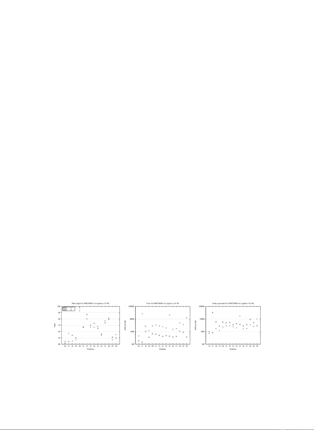
Fig. 8 shows the results of the two planners HSPr and HSP2 over the Logistics instances
16–30. The curves show the length of the solutions (left), the time required to find the
solutions (center), and the number of generated nodes (right). It is interesting to see that
HSPr generates more nodes than HSP2 and yet it takes roughly four times less time than
HSP2 to solve the problems. This follows from the faster evaluation of the heuristic. On the
other hand, the plans found by HSPr are often longer than those found by HSP2. Similar
results obtain for the logistics instances that are not shown in the figure.
Fig. 8. Comparison between HSPr versus HSP2 over Logistics instances 16–30. Curves show solution length (left),
time (center), and number of nodes generated (right).
B. Bonet, H. Geffner / Artificial Intelligence 129 (2001) 5–33 23
Fig. 9. Comparison between HSPr versus HSP2 over Gripper instances. Curves show solution length (left), solution
(center), and number of nodes generated (right).
Fig. 10. Comparison between HSPr versus HSP2 over Hanoi. Curves show solution length (left), solution (center),
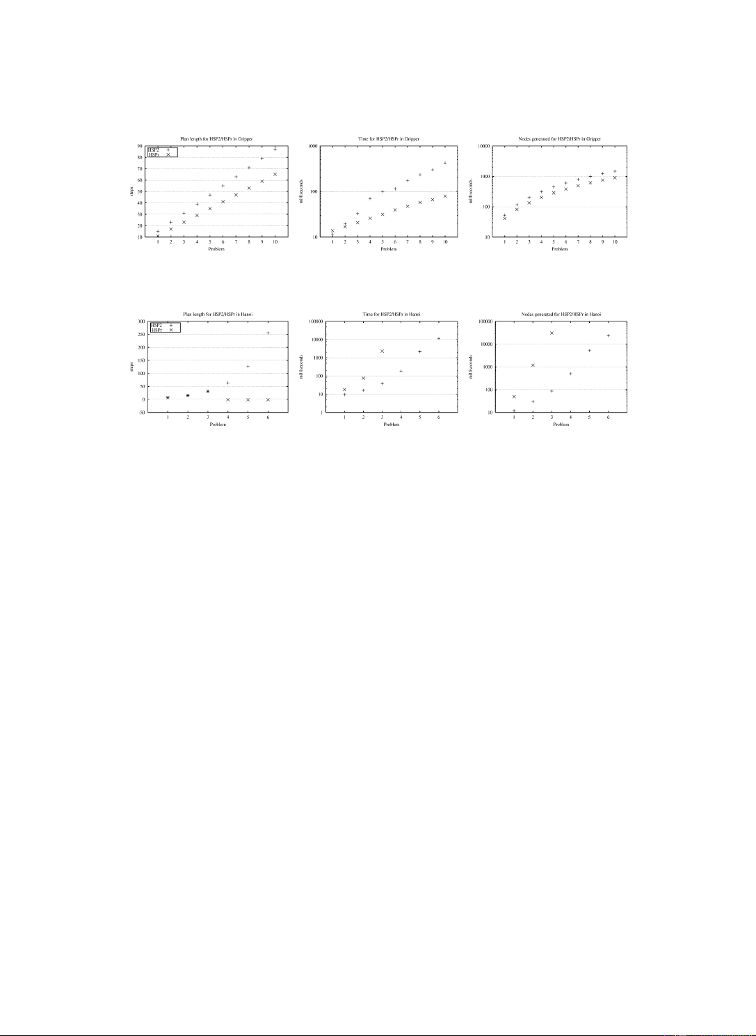
and number of nodes generated (right). Instance i has i + 2 disks. 6.5.2. Gripper
As shown in Fig. 9, a similar pattern arises in Gripper. Here HSPr generates slightly less
nodes than HSP2, but since it generates nodes faster, the time gap between the two planner
gets larger as the size of the problems grows. In this case, the solutions found by HSPr are
uniformly better than the solutions found by HSP2, and this difference grows with the size of the problems.
HSPr is also stronger than HSP2 in Puzzle where, unlike HSP2 (with W = 5), it solves the
last instance in the set (a 15-Puzzle instance). However, for the other three domains HSPr
does not improve on HSP2, and indeed, in two of these domains (Hanoi and Tire-World) it does significatively worse.
6.5.3. Hanoi and Tire-World
The results for Hanoi are shown in Fig. 10. HSPr solves the first three instances (up to
5 disks), but it does not solve the other three. Indeed, as it can be seen, in the first three
instances the time to find the solutions and the number of nodes generated grow much
faster in HSPr than in HSP2. The same situation arises in the Tire-World where HSP2 solves
all three instances and HSPr solves only the first one. The problems, as we mentioned
above, are two: spurious states generated in the regression search that are not detected by
the mutex mechanisms, and the lack of the ‘feedback’ provided by the recomputation of
the atom costs in every state. Indeed, errors in the estimated costs of atoms in HSP2 can be
corrected when they are recomputed; in HSPr, on the other hand, they are never recomputed.
So the recomputation of these costs has two effects, one that is bad (time overhead) and
one that is good (additional information). In domains where subgoals interact in complex
ways, the idea of a forward search in which atom costs are recomputed in every state as 24
B. Bonet, H. Geffner / Artificial Intelligence 129 (2001) 5–33
implemented in HSP2 will probably make sense; on the other hand, in domains where the
additive heuristic is adequate, the backward search with no recomputations as implemented in HSPr can be more efficient.
The results for the HSPr and HSP2 planners in the Tire-World show the same pattern as
Hanoi. Indeed, HSPr solves just the first instance, while HSP2 solves the three instances. As
we show below, however, part of the problem in this domain has to do with the spurious
states generated in the regression search.
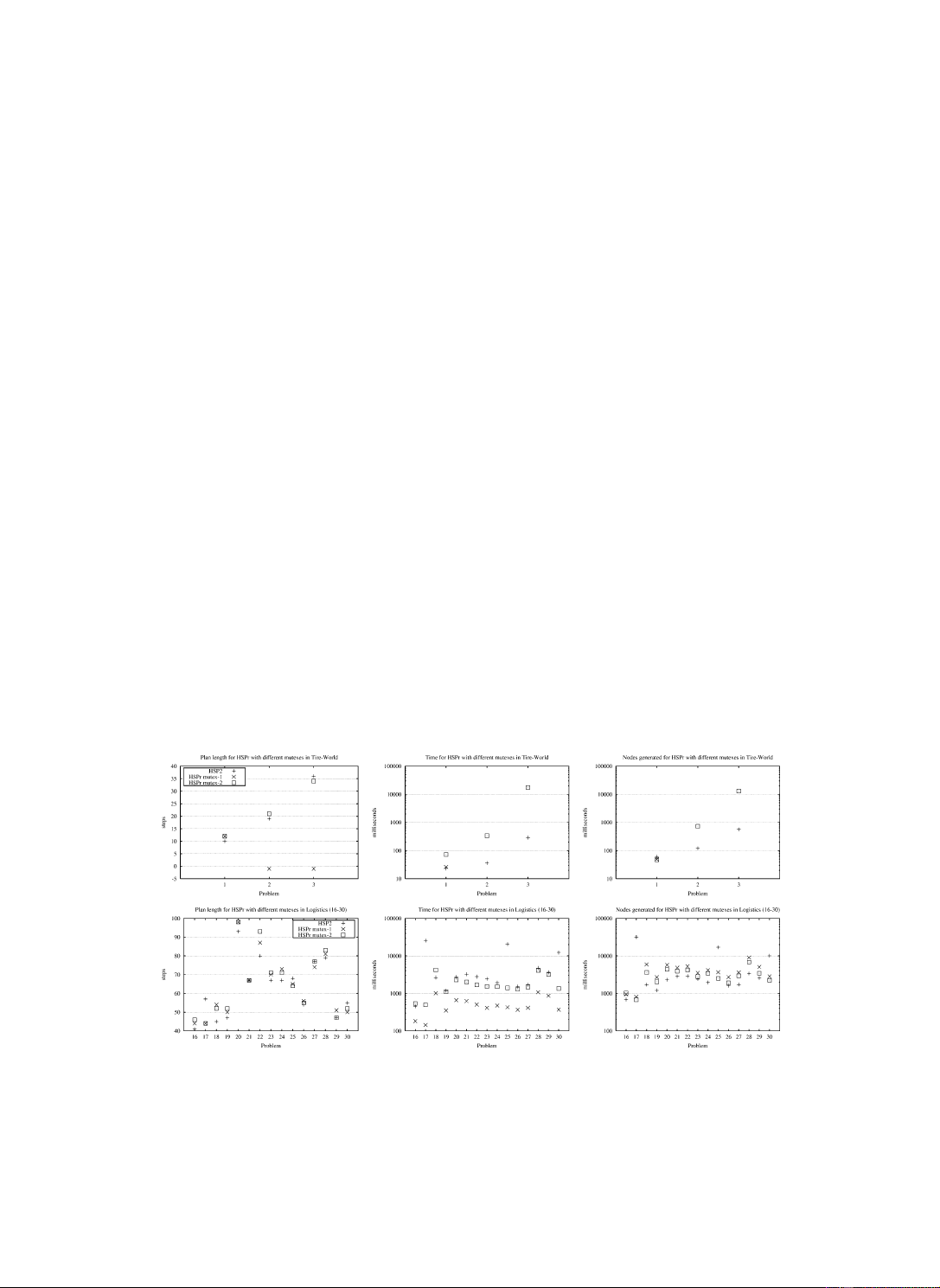
6.6. Improved mutex computation
The procedure used in HSPr to identify mutexes starts with a set M0 of potential mutexes
and then removes the ‘bad’ pairs from M0 until no ‘bad’ pair remains. A problem we have
detected with the definition in [4], which we have used here, is that the set of potential
mutexes M0 sometimes is not large enough and hence useful mutexes are lost. Indeed, we
performed experiments in which M0 is set to the collection of all atom pairs, and the same
procedure is applied to this set until no ‘bad’ pairs remains. In most of the domains, this
change didn’t yield a different behavior. However, there were two exceptions. While HSPr
solved only the first instance of the Tire-World, HSPr using the extended set of potential
mutexes solved the three instances. This shows that in this case HSPr was affected by the
problem of spurious states. On the other hand, in problems like logistics, the new set M0
leads to a much larger set of mutexes M∗ that are not as useful and yet have to be checked
in all the states generated. This slows down node generation with no compensating gain
thus making HSPr several times slower. The corresponding curves are shown in Fig. 11,
where ‘mutex-1’ and ‘mutex-2’ correspond to the original and extended definition of the
set M0 of potential mutexes. Since, the benefits appear to be more important than the loses,
the extended definition seems worthwhile and we will make it the default option in the next
version of HSPr. However, since for the reasons above, the new mechanism is not complete
Fig. 11. Impact of original versus extended definition of the set M0 of potential mutexes in Tire-World and Logistics.
Tài liệu liên quan:
-

Ung dung game hoa trong cac chien dich MKT
27 14 -

Bao cao Chi so TMDT Viet Nam 2025
30 15 -
Thông tư quy định về việc phân quyền, phân cấp và phân định thẩm quyền quản lý nhà nước về giáo dục cho chính quyền địa phương
31 16 -
Nghị quyết về phát huy các giá trị di sản văn hóa gắn với phát triên du lịch bền vững tỉnh Khánh Hòa đến năm 2025, định hướng đến năm 2030
34 17 -
Quyết định phê duyệt Chiến lược phát triển du lịch Việt Nam đến năm 2030
20 10