Principles of economics chapter 6
Principles of economics chapter 6
Môn: Kinh tế vi mô (ECO111) 7 tài liệu
Trường: Trường Đại học FPT Hà Nội 62 tài liệu
Tác giả:


Preview text:
lOMoARcPSD|36041561
PowerPoint Lecture Notes for Chapter 6:
Supply, Demand, and Government Policies
Principles of Economics 5th edition, by N. Gregory Mankiw
Premium PowerPoint Slides by Ron Cronovich
This chapter builds on the previous two (supply & demand and C H A P T E R 6
elasticity). Students who learned those chapters well usually do
Su p p ly, Dem an d , an d
not have much difficulty with the material in Chapter 6. This G overn m en t Policies
chapter can usually be covered in about 90 minutes of class time. EcP Po R R I Nn N C C I o P P L Em S S O O Fi F cs N. N Gr G egory Ma M nkiw
I have combined the analysis of price ceilings with the rent control
example, and I’ve combined the analysis of price floors with the Premium PowerPoint Slides by Ron Cronovich
minimum wage example. (In contrast, the textbook presents a
© 2009 South-Western, a part of Cengage Learning, all rights reserved
generic analysis of price ceilings, then the rent control example,
then a generic analysis of price floors, then the minimum wage).
Most students learn new concepts better in the context of a
specific example rather than a generic analysis, and combining
them in this way saves class time.
Here’s an idea you might consider:
At the end of the class session just prior to the one in which you
begin to cover this chapter, ask students to take out a piece of
blank paper, and write down whether they think the minimum
wage should be increased, and their reason(s). Tell them not to
write their names (you want them to be candid), and have them
leave their pieces of paper in a pile as they exit the classroom.
Later, divide the papers into two groups based on whether they
support or oppose increasing the minimum wage. In this
PowerPoint file, immediately after this slide, insert new two slides,
titling them “Your reasons for raising the minimum wage” and
“Your reasons for not raising the minimum wage.” Summarize on
each slide the most common reasons students gave. Begin the
class session by showing them the results of this impromptu
survey (how many students responded each way, and the most
common reasons). Tell those students that support a minimum
wage increase that their thinking represents that of many educated
non-economists. But tell them that economics offers another
perspective, and this is something they will learn in this chapter.
If you do this, then I recommend rearranging the slides a bit so
that the price floor/minimum wage slides come BEFORE the price ceiling/rent control slides.
Downloaded by Nga T??ng (ngahuong55@gmail.com) lOMoARcPSD|36041561 In th is ch ap ter,
When we talk about how a policy “affects the market
look for th e an sw ers to th ese q u estion s:
outcome,” we mean the policy’s impact on the price and
§ What are price ceilings and price floors?
quantity of the good and therefore on the market’s allocation
What are some examples of each?
§ How do price ceilings and price floors affect
of resources. The concluding slide elaborates on this a bit. market outcomes?
§ How do taxes affect market outcomes?
How do the effects depend on whether
the tax is imposed on buyers or sellers?
§ What is the incidence of a tax?
What determines the incidence? 4
G overn men t Policies Th at Alter th e
This slide outlines the chapter.
Private M ark et Ou tcom e § Price controls
§ Price ceiling: a legal maximum on the price
of a good or service Example: rent control
§ Price floor: a legal minimum on the price of
a good or service Example: minimum wage § Taxes
§ The govt can make buyers or sellers pay a
specific amount on each unit bought/sold. W W e e w w iillll u u se se tth h e e s s u su u p p p p lly/ y/ d d e e ma ma n n d d mo mo d d e e ll tto o se se e e h h o o w w e e a a c c h ch h p p o o lliicy cy a a ffffe e ct ct s s s tth h e e ma ma rke rke tt o o u u ttco co co me me (t (t he pri ri ce ce b b u u ye ye rs pa a y, y, the p p rice se se lllers rs re re ceiive ve , a a nd d e e q’’m qu u antitty). y).
SUPPLY, DEMAND, AND GOVERNMENT POLICIES 5
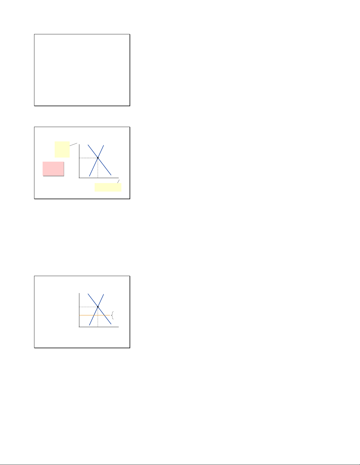
We start by analyzing the effects of a price ceiling. The
EXAM PLE 1: Th e M ark e t for Ap artm en ts
most common example is rent control, so we do the analysis P Rental S price of
in the context of this example. apts $800 Eq’m w/o pri ri ce
We begin by showing the market for apartments in controls D Q
equilibrium (before the government imposes any price 300 Quantity of controls). apartments
SUPPLY, DEMAND, AND GOVERNMENT POLICIES 6
Downloaded by Nga T??ng (ngahuong55@gmail.com) lOMoARcPSD|36041561
H ow Price Ceilin gs Affect M ark et O u tcomes
When some students see this for the first time, they wonder A price ceiling
why the price ceiling does not result in a surplus. P S above the Price eq’m price is $1000 ceiling not binding – has no effect $800
When the price ceiling is above the equilibrium price, the on the market outcome.
equilibrium price is still perfectly legal. Just because D Q
landlords are allowed to charge $1000 rent doesn’t mean 300
they will – if they do, they won’t be able to rent all of their
SUPPLY, DEMAND, AND GOVERNMENT POLICIES 7
apartments – a surplus will result, causing downward
pressure on the price (rent). There’s no law that prevents the
price (rent) from falling, so it does fall until the surplus is
gone and equilibrium is reached (at P = $800 and Q = 300).
H ow Price Ceilin gs Affect M ark et O u tcomes
In this case, the price ceiling is binding. The eq’m price P S ($800) is above the ceiling and
In the new equilibrium with the price ceiling, the actual price therefore illegal. $800
(rent) of an apartment will be $500. It won’t be more than The ceiling is a binding Price $500 constraint ceiling
that, because any higher price is illegal. It won’t be less than on the price, shortage D causes a Q
$500, because the shortage would be even larger if the price 250 400 shortage. were lower.
SUPPLY, DEMAND, AND GOVERNMENT POLICIES 8
The actual quantity of apartments rented equals 250, and
there is a shortage equal to 150 (the difference between the
quantity demanded, 400, and the quantity supplied, 250).
H ow Price Ceilin gs Affect M ark et O u tcomes
In this slide, the equilibrium price ($800) and price ceiling
($500) are the same as on the preceding slides, but supply In the long run, P S supply and
and demand are more price-elastic than before, and the demand are more $800
shortage that results from a binding price ceiling is larger. price-elastic. Price So, the $500 ceiling shortage shortage is larger. DQ 150 450
SUPPLY, DEMAND, AND GOVERNMENT POLICIES 9
Downloaded by Nga T??ng (ngahuong55@gmail.com) lOMoARcPSD|36041561
Sh ortages an d Rationing
The last two bullets discuss “efficiency” in the context of
§ With a shortage, sellers must ration the goods
rationing goods to those buyers who value them most highly. among buyers.
§ Some rationing mechanisms: (1) Long lines
This concept will be explored further in the following
(2) Discrimination according to sellers’ biases § chapter.
These mechanisms are often unfair, and inefficient:
the goods do not necessarily go to the buyers who value them most highly.
§ In contrast, when prices are not controlled,
the rationing mechanism is efficient (the goods
go to the buyers that value them most highly)
and impersonal (and thus fair).
SUPPLY, DEMAND, AND GOVERNMENT POLICIES 10
Now we switch gears and look at the effects of a price floor.
EXAM PLE 2: Th e M ark et for Un sk illed La b or
We illustrate this concept using the common textbook W Wage S paid to example – the minimum wage. unskilled workers $4 Eq’m w/o pri ri ce
This may be the first time students have seen a supply- controls D L
demand diagram of the labor market. It might be useful to 500 Quantity of
note that the “price” of labor is simply the wage, which we unskilled workers
SUPPLY, DEMAND, AND GOVERNMENT POLICIES 11
measure on the vertical axis of our supply-demand diagram.
Along the horizontal axis, we measure the quantity of labor
(number of workers). The demand for unskilled labor comes
from firms. The supply comes from workers.
We focus on unskilled labor because the minimum wage is
not relevant for higher skilled, higher wage workers.
H ow Price Floors Affect M ark et O u tcom es
Some students may wonder why the $3 price floor does not A price floor
cause a shortage. After all, at a wage of $3, the quantity of W S below the eq’m price is
unskilled workers that firms wish to hire exceeds the not binding – $4 has no effect
quantity of unskilled workers that are looking for jobs. on the market Price $3 outcome. floor D L
But the minimum wage law does not stop the wage from 500
rising above $3. So, in response to this shortage, the wage
SUPPLY, DEMAND, AND GOVERNMENT POLICIES 12
will rise until the shortage disappears – which occurs at the
equilibrium wage of $4. The equilibrium wage is perfectly
legal when the price floor (i.e. minimum wage) is below it.
Downloaded by Nga T??ng (ngahuong55@gmail.com) lOMoARcPSD|36041561
H ow Price Floors Affect M ark et O u tcom es
Now, the minimum wage exceeds the equilibrium wage. labor The eq’m wage ($4)
The equilibrium wage (or any wage below $5) is illegal. W surplus S is below the floor Price $5 and therefore floor illegal. $4
In this case, the actual wage will be $5. It will not be lower, The floor is a binding constraint
because any lower wage is illegal. It will not be higher, on the wage, D causes a L
because at any higher wage, the surplus would be even 400 550 surplus (i.e., unemployment).
greater. The actual number of unskilled workers with jobs
SUPPLY, DEMAND, AND GOVERNMENT POLICIES 13
equals 400. 550 want jobs, but firms are only willing to hire
400, leaving a surplus (i.e. unemployment) of 150 workers.
A surplus of anything – especially labor – represents wasted resources. Th e M inim um Wage Min wage laws unemp- do not affect W loyment S Min. highly skilled $5 wage workers. They do affect $4 teen workers. Studies: A 10% increase in the min wage D L raises teen 400 550 unemployment by 1-3%.
SUPPLY, DEMAND, AND GOVERNMENT POLICIES 14
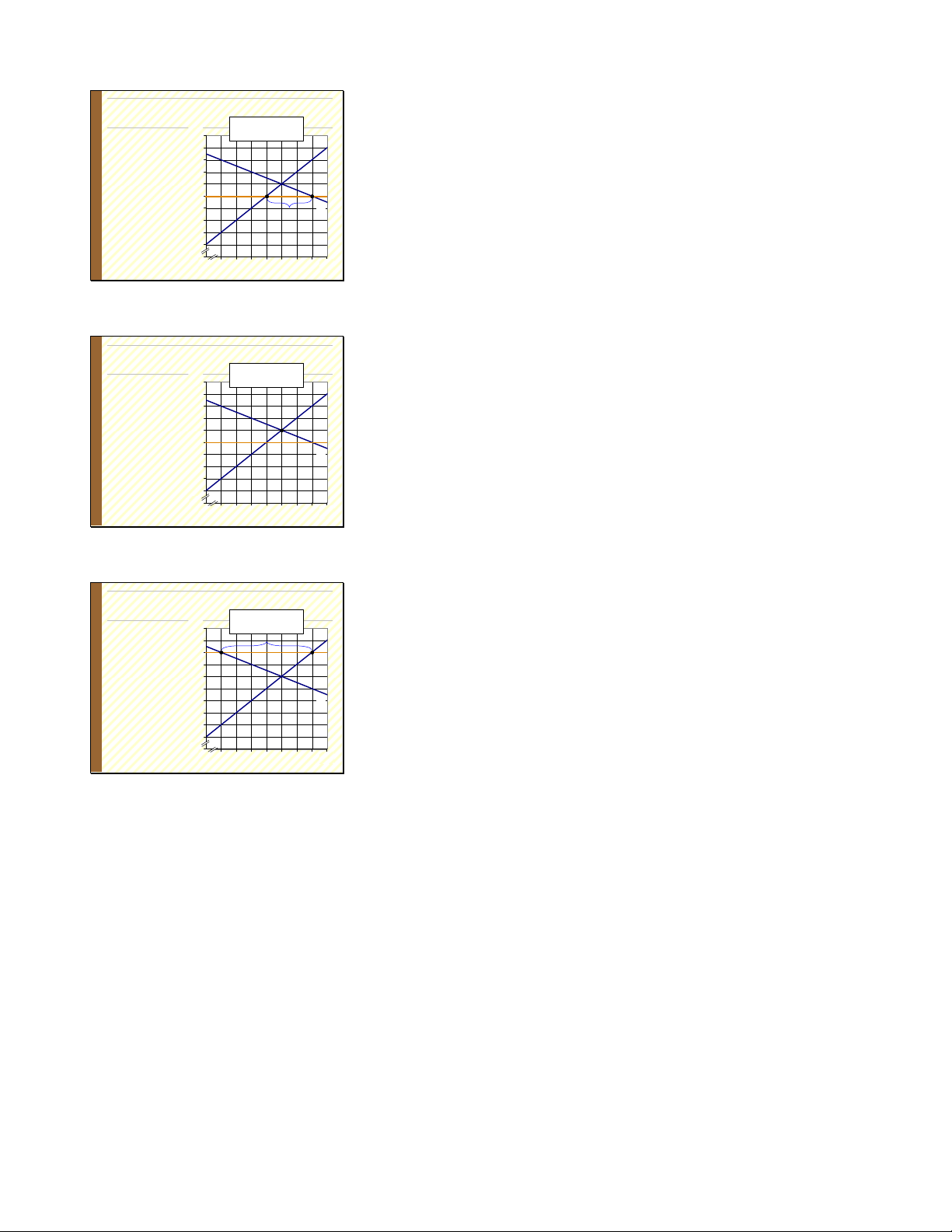
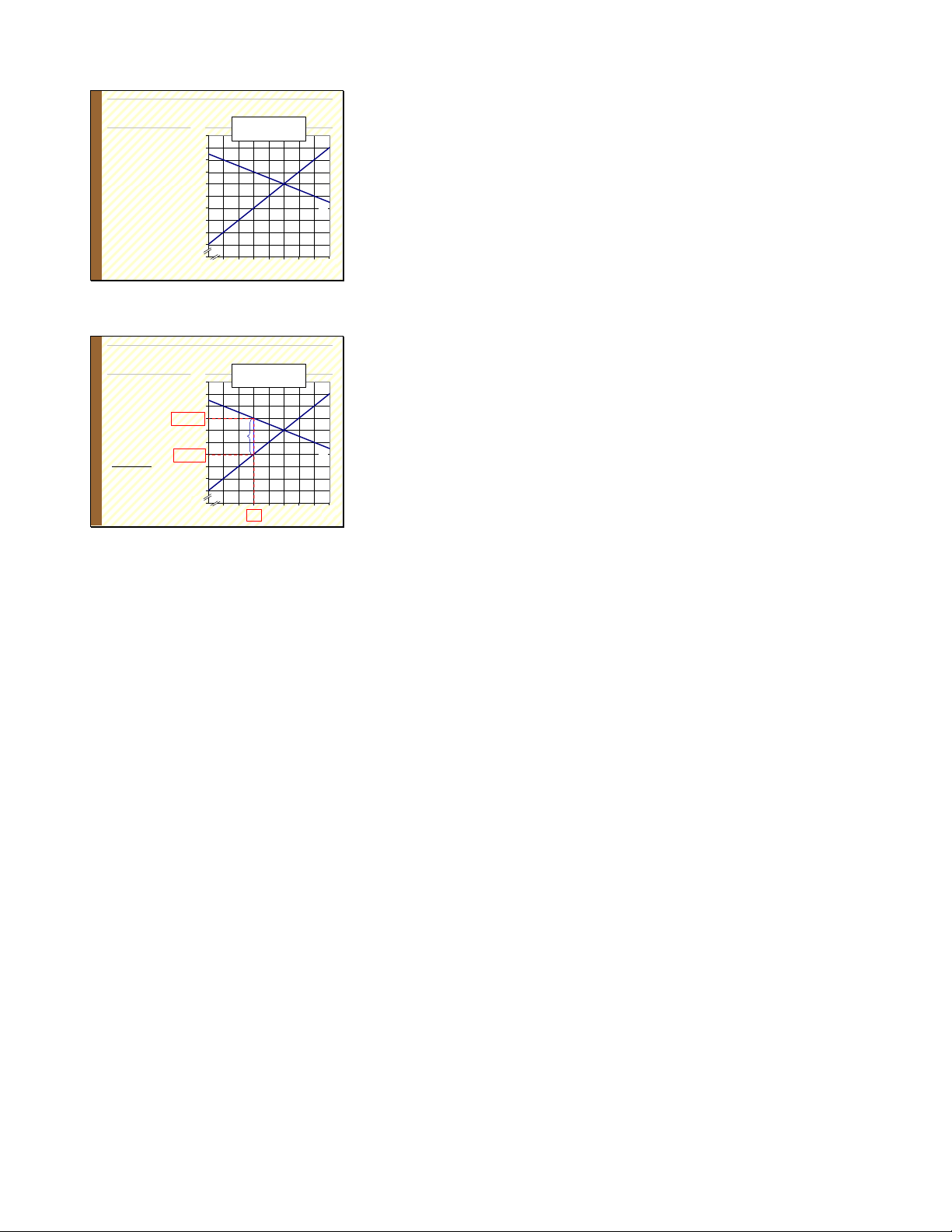
A good exercise to break up the lecture, engage students, and A A C C T I V V E E L L E E A A R R N I N G G 1 Price con trols The market for assess their learning so far. 140 P hotel rooms S 130 Determine 120 effects of: 110 A. $90 price 100 ceiling 90 B. $90 price 80 D floor 70 60 C. $120 price 50 floor
40050 60 70 80 90 100 110 120 130 Q15
Downloaded by Nga T??ng (ngahuong55@gmail.com) lOMoARcPSD|36041561 A A C C T I V V E E L L E E A A R R N I N G G 1 A. $90 $90 p rice ceilin g The market for 140 P hotel rooms The price S 130 falls to $90. 120 Buyers 110 demand 100 120 rooms, Price ceiling 90 sellers supply 80 D 90, leaving a shortage = 30 70 shortage. 60 50
40050 60 70 80 90 100 110 120 130 Q16 A A C C T I V V E E L L E E A A R R N I N G G 1 B. $90 $ 90 p rice floor The market for 140 P hotel rooms Eq’m price is S 130 above the floor, 120 so floor is not 110 binding. 100 P = $100, 90 Q = 100 rooms. Price floor 80 D 70 60 50
40050 60 70 80 90 100 110 120 130 Q17 A A C C T I V V E E L L E E A A R R N I N G G 1 C. $12 $ 0 120 price floor The market for 140 P hotel rooms The price S 130 rises to $120. surplus = 60 120 Buyers Price floor 110 demand 100 60 rooms, 90 sellers supply 80 D 120, causing a 70 surplus. 60 50
40050 60 70 80 90 100 110 120 130 Q18
Downloaded by Nga T??ng (ngahuong55@gmail.com) lOMoARcPSD|36041561
RE: the last bullet “price controls often hurt the poor more
Evalu atin g Price Con trols
§ Recall one of the Ten Principles from Chapter 1:
than help them.” We have seen that the minimum wage can
Markets are usually a good way
to organize economic activity.
cause job losses, and rent control can reduce the quantity and
§ Prices are the signals that guide the allocation of
quality of affordable housing. Both policies make the poor
society’s resources. This allocation is altered
when policymakers restrict prices. worse off.
§ Price controls often intended to help the poor,
but often hurt more than help.
It might be worth reminding students that our analysis has
SUPPLY, DEMAND, AND GOVERNMENT POLICIES 19
been in the context of a world without market failures.
Subsequent chapters (except in the macro split) will
introduce situations in which government intervention can
improve on the private market outcome. However, even in
such cases, the appropriate policy is usually something other than a direct price control.
The slides in this section have been revised from the Taxes
§ The govt levies taxes on many goods & services
previous edition. They now better explain why a tax on
to raise revenue to pay for national defense, public schools, etc.
buyers shifts D down by the amount of the tax, and why a
§ The govt can make buyers or sellers pay the tax.
tax on sellers shifts S up by the amount of the tax.
§ The tax can be a % of the good’s price,
or a specific amount for each unit sold.
§ For simplicity, we analyze per-unit taxes only.
SUPPLY, DEMAND, AND GOVERNMENT POLICIES 20
EXAM PLE 3: Th e Mark et for Pizza Eq’m w/o tax P S1 $10.00 D1 Q 500
SUPPLY, DEMAND, AND GOVERNMENT POLICIES 21
Downloaded by Nga T??ng (ngahuong55@gmail.com) lOMoARcPSD|36041561 A Tax on Bu yers
NOTE: On this and subsequent slides, “PB” denotes the Th H e e np cr ei ec , e a b t u a y x e ors n p b a u y y ers Effects of a $1.50 per
price buyers pay and “PS” denotes the price sellers receive. is n hi o ftw s t$ h1 e. 5 D0 D c h cui u g rvh vee e r d d t oh o a w n n unit tax on buyers th be y tm th a e r k a e mt m op our u i nc nt e o oP f t . t P he tax.
(The Chapter 8 PowerPoint uses the same notation for the
P would have to fall S1 by $1.50 to make welfare analysis of taxes.) $10.00 buyers willing Tax to buy same Q as before. $8.50 D1
E.g., if P falls
The government makes buyers pay a $1.50 on each pizza from $10.00 to $8.50, D2 buyers still willing to Q 500 purchase 500 pizzas.
they purchase. The new demand curve (in red, labeled D2)
SUPPLY, DEMAND, AND GOVERNMENT POLICIES 22
reflects buyers’ demand as a function of the after-tax price.
The original demand curve (D1) still reflects buyers’ demand
as a function of the total price – inclusive of the tax.
Thus, buyers’ demand hasn’t really changed: at each
quantity, the height of the original (blue) D curve is still the
maximum that buyers will pay for that quantity, while the
height of the new (red) D curve is the maximum that buyers
will pay sellers for that quantity, given that buyers also must
pay the tax. At any Q, the vertical distance between the blue
and red D curves equals the tax.
(If this were a percentage tax rather than a per-unit tax, the
new D curve would not be parallel to the old one, it would be
flatter: a tax of a given percentage would be a larger dollar
amount at high prices than at low prices, so the downward
shift would be greater in absolute terms when P is high than
when it is low. This is the type of complexity we avoid by working with per-unit taxes.) A Tax on Bu yers New eq’m: Effects of a $1.50 per unit tax on buyers Q = 450 P Sellers S1 P = $11.00 B receive Tax P = $9.50 S $10.00 P = $9.50 Buyers pay S P = $11.00 B D1 Difference D between them 2 Q = $1.50 = tax 450 500
SUPPLY, DEMAND, AND GOVERNMENT POLICIES 23
Downloaded by Nga T??ng (ngahuong55@gmail.com) lOMoARcPSD|36041561
The In cid en ce of a Tax:
“Market participants” simply means buyers and sellers.
how the burden of a tax is shared among market participants P In our S1 example, P = $11.00 B Tax buyers pay $10.00 $1.00 more, P = $9.50 S sellers get D $0.50 less. 1 D2 Q 450 500
SUPPLY, DEMAND, AND GOVERNMENT POLICIES 24 A Tax on Sellers
The government makes sellers pay a $1.50 on each pizza Effects of a $1.50 per The tax effectively raises
they sell. The new, red supply curve reflects sellers’ supply unit tax on sellers sellers’ costs by P S $1.50 per pizza. 2
as a function of the after-tax price. $11.50 Tax S1 Sellers will supply 500 pizzas $10.00 only if
P rises to $11.50, to compensate for D1 this cost increase.
Hence, a tax on sellers shifts the Q 500
S curve up by the amount of the tax.
SUPPLY, DEMAND, AND GOVERNMENT POLICIES 25 A Tax on Sellers New eq’m: Effects of a $1.50 per unit tax on sellers Q = 450 P S2 Buyers pay S1 P = $11.00 B P = $11.00 B Tax $10.00 Sellers P = $9.50 receive S P = $9.50 S D1 Difference between them Q = $1.50 = tax 450 500
SUPPLY, DEMAND, AND GOVERNMENT POLICIES 26
Downloaded by Nga T??ng (ngahuong55@gmail.com) lOMoARcPSD|36041561
The O utcom e Is th e Sam e in Both Cases!
Whether the government makes buyers or sellers pay the tax,
The effects on P and Q, and the tax incidence are the
all of the effects are the same:
same whether the tax is imposed on buyers or sellers! What matters P
- the price buyers pay rises (in this case to $11) is this: S1 P = $11.00 B Tax A tax drives
- the price sellers receive falls (to $9.50) $10.00 a wedge P = $9.50 between the S
- the equilibrium quantity falls (to 450) price buyers D1 pay and the
- the incidence of the tax is the same (here, buyers pay $1 price sellers Q receive. 450 500
of the tax, while sellers pay $.50 of the tax on each unit)
SUPPLY, DEMAND, AND GOVERNMENT POLICIES 27
This should make sense if students think it through: A tax
on buyers means buyers will have to pay more, which causes
their demand to fall. The fall in demand hurts sellers,
forcing them to reduce their price. Similarly, a tax on sellers
is like a cost increase, and sellers pass along a portion of that
increase to buyers in the form of higher prices.
The equivalence of taxes on buyers and taxes on sellers
means that we can ignore whether the tax is imposed on
buyers or sellers. All that matters is the size of the tax.
So, in future problems, we can think of the tax as a wedge
between the price buyers pay and the price sellers receive.
On a supply-demand diagram, this wedge is a vertical line
segment (shown in green on this graph). You can think of
taking a toothpick the size of the tax and wedging it between
the S and D curves. The quantity at which the toothpick fits
just snuggly is the new equilibrium quantity. Students will
have a chance to practice this in a moment with an exercise.
One last remark: Someone once said “if you want less of
something, tax it.” A tax on any good or service causes a fall
in its quantity. This is because people respond to incentives:
the tax gives buyers an incentive to buy less and gives sellers an incentive to produce less.
Downloaded by Nga T??ng (ngahuong55@gmail.com) lOMoARcPSD|36041561
These are the same supply and demand curves used in the A A C C T I V V E E L L E E A A R R N I N G G 2 Effects of a tax The market for previous exercise. 140 P hotel rooms Suppose govt S 130 imposes a tax 120 on buyers of 110 $30 per room. 100 Find new 90
Q, P , P , 80 D B S and incidence 70 of tax. 60 50
40050 60 70 80 90 100 110 120 130 Q
First, the equilibrium quantity is the quantity where P A A C C T I V V E E L L E E A A R R N I N G G 2 B – PS = An swers The market for $30. This quantity is 80. 140 P hotel rooms S 130 Q = 80 120 P = $110 B P = 110 B
Next, to find PB, start at Q=80 and go up to the demand 100 P = $80 S Tax 90 curve to see that PB = $110. P = 80 D Incidence S 70 buyers: $10 60 sellers: $20 50 To find P 40
S, start at Q=80 and go up to the supply curve to see
050 60 70 80 90 100 110 120 130 Q that PS = $80.
To find incidence, just compare PB and PS to the no-tax equilibrium price, $100.
Downloaded by Nga T??ng (ngahuong55@gmail.com) lOMoARcPSD|36041561
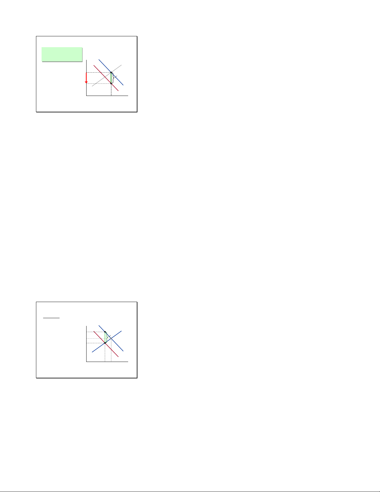
We have just seen that tax incidence is not affected by
Elasticity an d Tax In cid en ce
CASE 1: Supply is more elastic than demand
whether the government makes buyers or sellers pay the tax. P It’s easier
So what, then, does determine tax incidence? Turns out it’s for sellers than buyers Buyers’ share P than buyers B S to leave the
elasticity – specifically, the price elasticities of supply and of tax burden to leave the Tax market. Price if no tax So buyers demand. Sellers’ share bear most of P bear most of S of tax burden the burden of the tax. D of the tax. Q
There are two cases: 1) supply is more price-elastic than
SUPPLY, DEMAND, AND GOVERNMENT POLICIES 30
demand (this slide), and 2) demand is more price-elastic than supply (next slide).
When supply is more price-elastic than demand, sellers are
relatively more responsive to changes in price, and the
supply curve is less steep than the demand curve. Buyers
have relatively fewer alternatives, so they have to “eat” most
of the price increase caused by the imposition of the tax.
As the textbook puts it, sellers can more easily leave the
market in response to the tax than can buyers. Thus, buyers
are stuck bearing most of the burden of the tax.
The size of the tax is the same in this diagram as in the one
Elasticity an d Tax In cid en ce
CASE 2: Demand is more elastic than supply on the preceding slide. It’s easier P It’s easier S for buyers Buyers’ share than sellers of tax burden PB to leave the
When demand is more price-elastic than supply, buyers are market. Price if no tax market. Tax Sellers bear
relatively more price-sensitive, and the demand curve is less Sellers’ share most of the of tax burden P burden of S burden of
steep than the supply curve. Buyers have relatively more D the tax. Q
alternatives, so they can avoid most of the tax. Sellers are
SUPPLY, DEMAND, AND GOVERNMENT POLICIES 31
less flexible, so they have to “eat” a greater share of the price increase caused by the tax. From the textbook:
Buyers can more easily leave the market than sellers in
response to the tax. Thus, sellers end up with most of the burden of the tax.
Downloaded by Nga T??ng (ngahuong55@gmail.com) lOMoARcPSD|36041561
This case study shows students an interesting real-world
CASE STUD Y: Wh o Pays th e Lu xu ry Tax?
§ 1990: Congress adopted a luxury tax on yachts,
example of the material they just learned.
private airplanes, furs, expensive cars, etc.
§ Goal of the tax: raise revenue from those
who could most easily afford to pay –
If you’re pressed for time, it is probably safe to skip it and let wealthy consumers.
§ But who really pays this tax?
students read it on their own. It does not introduce any new
concepts, and most students do not find it difficult to read.
SUPPLY, DEMAND, AND GOVERNMENT POLICIES 32
Demand for yachts (and other luxury items) is price-elastic:
CASE STUD Y: Wh o Pays th e Lu xu ry Tax?
if the price of yachts rises, rich consumers can easily avoid The market for yachts Dema ma nd is price-e -e lastic. P S
the tax by spending their millions on some other luxury item. In the sh sh ort ru ru n, Buyers’ share supply is inelastic. of tax burden P supply is inelastic. B Tax Hence,
Supply of yachts is less elastic, especially in the short run. It comp mp anies Sellers’ share that build of tax burden PS yachts pay
is difficult for the companies that build yachts to re-tool their D yachts pay most st of Q the tax. x.
factories and reeducate their workers to produce some other
SUPPLY, DEMAND, AND GOVERNMENT POLICIES 33 product.
Hence, companies that build yachts pay most of the tax, and
the rich pay relatively little of it.
The same is true for taxes on other luxury items.
CO NCLUSION : G overn m en t Policie s an d
Recall one of the 10 principles from Chapter 1: Markets are
th e Allocation of Resou rces
usually a good way to organize economic activity. This
§ Each of the policies in this chapter affects the
allocation of society’s resources.
means that, in absence of market failures (which we will
§ Example 1: A tax on pizza reduces eq’m Q.
With less production of pizza, resources
learn more about in later chapters), the allocation of
(workers, ovens, cheese) will become available to other industries.
resources resulting from the free market equilibrium is
§ Example 2: A binding minimum wage causes
a surplus of workers, a waste of resources.
optimal. Hence, government policies which alter this
§ So, it’s important for policymakers to apply such
allocation tend to make the economy worse off. policies very carefully.
SUPPLY, DEMAND, AND GOVERNMENT POLICIES 34
When we study market failures later, we will see that
government policies can – in principle – improve on the
market’s allocation of resources, and make society better off.
First, though, we need to learn how to measure the impact of
government policies like taxes on society’s well-being, as
well as define what, exactly, we mean by “well-being.” This
field of study, called “welfare economics,” is the topic of the following three chapters.
Downloaded by Nga T??ng (ngahuong55@gmail.com) lOMoARcPSD|36041561 CH APTER SUMM ARY
§ A price ceiling is a legal maximum on the price of a
good. An example is rent control. If the price
ceiling is below the eq’m price, it is binding and causes a shortage.
§ A price floor is a legal minimum on the price of a
good. An example is the minimum wage. If the
price floor is above the eq’m price, it is binding
and causes a surplus. The labor surplus caused
by the minimum wage is unemployment. 35 CH APTER SUMM ARY
§ A tax on a good places a wedge between the price
buyers pay and the price sellers receive, and
causes the eq’m quantity to fall, whether the tax is imposed on buyers or sellers.
§ The incidence of a tax is the division of the burden
of the tax between buyers and sellers, and does
not depend on whether the tax is imposed on buyers or sellers.
§ The incidence of the tax depends on the price
elasticities of supply and demand. 36
Downloaded by Nga T??ng (ngahuong55@gmail.com)