Sample size for market research - Tài liệu tham khảo | Đại học Hoa Sen

Sample size for market research - Tài liệu tham khảo | Đại học Hoa Sen và thông tin bổ ích giúp sinh viên tham khảo, ôn luyện và phục vụ nhu cầu học tập của mình cụ thể là có định hướng, ôn tập, nắm vững kiến thức môn học và làm bài tốt trong những bài kiểm tra, bài tiểu luận, bài tập kết thúc học phần, từ đó học tập tốt và có kết quả

Determining Sample Size Page 2
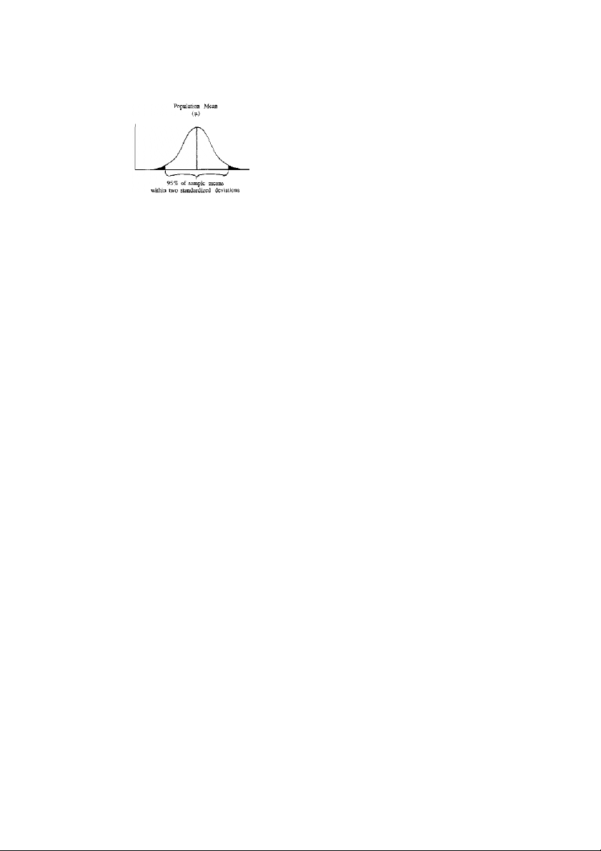
Figure 1. Distribution of Means for Repeated
Samples.
Degree Of Variability
The third criterion, the degree of variability in the
attributes being measured refers to the distribution of
attributes in the population. The more heterogeneous
a population, the larger the sample size required to
obtain a given level of precision. The less variable
(more homogeneous) a population, the smaller the
sample size. Note that a proportion of 50% indicates
a greater level of variability than either 20% or 80%.
This is because 20% and 80% indicate that a large
majority do not or do, respectively, have the attribute
of interest. Because a proportion of .5 indicates the
maximum variability in a population, it is often used
in determining a more conservative sample size, that
is, the sample size may be larger than if the true
variability of the population attribute were used.
STRATEGIES FOR DETERMINING
SAMPLE SIZE
There are several approaches to determining the
sample size. These include using a census for small
populations, imitating a sample size of similar studies,
using published tables, and applying formulas to
calculate a sample size. Each strategy is discussed
below.
Using A Census For Small Populations
One approach is to use the entire population as
the sample. Although cost considerations make this
impossible for large populations, a census is attractive
for small populations (e.g., 200 or less). A census
eliminates sampling error and provides data on all the
individuals in the population. In addition, some costs
such as questionnaire design and developing the
sampling frame are "fixed," that is, they will be the
same for samples of 50 or 200. Finally, virtually the
entire population would have to be sampled in small
populations to achieve a desirable level of precision.
Using A Sample Size Of A Similar Study
Another approach is to use the same sample size
as those of studies similar to the one you plan.
Without reviewing the procedures employed in these
studies you may run the risk of repeating errors that
were made in determining the sample size for another
study. However, a review of the literature in your
discipline can provide guidance about "typical" sample
sizes which are used.
Using Published Tables
A third way to determine sample size is to rely on
published tables which provide the sample size for a
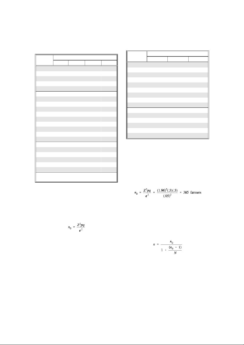
given set of criteria. Table 1 and Table 2 present
sample sizes that would be necessary for given
combinations of precision, confidence levels, and
variability. Please note two things. First, these
sample sizes reflect the number of responses,obtained
and not necessarily the number of surveys mailed or
interviews planned (this number is often increased to
compensate for nonresponse). Second, the sample
sizes in Table 2 presume that the attributes being
measured are distributed normally or nearly so. If
this assumption cannot be met, then the entire
population may need to be surveyed.
Using Formulas To Calculate A Sample Size
Although tables can provide a useful guide for
determining the sample size, you may need to
calculate the necessary sample size for a different
combination of levels of precision, confidence, and
variability. The fourth approach to determining
sample size is the application of one of several
formulas (Equation 5 was used to calculate the
sample sizes in Table 1 and Table 2).
Determining Sample Size Page 3
Table 1. Sample size for 3%, 5%, 7% and 10%
Precision Levels Where Confidence Level is 95% and
P=.5.
Size of Sample Size (n) for Precision (e) of:
Population
3% 5% 7% 10%
500 a 222 145 83
600 a 240 152 86
700 a 255 158 88
800 a 267 163 89
900 a 277 166 90
1,000 a 286 169 91
2,000 714 333 185 95
3,000 811 353 191 97
4,000 870 364 194 98
5,000 909 370 196 98
6,000 938 375 197 98
7,000 959 378 198 99
8,000 976 381 199 99
9,000 989 383 200 99
10,000 1,000 385 200 99
15,000 1,034 390 201 99
20,000 1,053 392 204 100
25,000 1,064 394 204 100
50,000 1,087 397 204 100
100,000 1,099 398 204 100
>100,000 1,111 400 204 100
a = Assumption of normal population is poor (Yamane,
1967). The entire population should be sampled.
Formula For Calculating A Sample For
Proportions
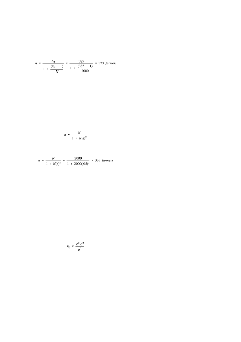
For populations that are large, Cochran (1963:75)
developed the Equation 1 to yield a representative
sample for proportions.
Which is valid where n
0
is the sample size, Z
2
is the
abscissa of the normal curve that cuts off an area at
the tails (1 - equals the desired confidence level,
e.g., 95%)
1
, e is the desired level of precision, p is the
estimated proportion of an attribute that is present in
the population, and q is 1-p. The value for Z is
found in statistical tables which contain the area
under the normal curve.
To illustrate, suppose we wish to evaluate a state-
Table 2. Sample size for 5%, 7% and 10% Precision
Levels Where Confidence Level is 95% and P=.5.
Size of Sample Size (n) for Precision (e) of:
Population
5% 7% 10%
100 81 67 51
125 96 78 56
150 110 86 61
175 122 94 64
200 134 101 67
225 144 107 70
250 154 112 72
275 163 117 74
300 172 121 76
325 180 125 77
350 187 129 78
375 194 132 80
400 201 135 81
425 207 138 82
450 212 140 82
wide Extension program in which farmers were
encouraged to adopt a new practice. Assume there is
a large population but that we do not know the
variability in the proportion that will adopt the
practice; therefore, assume p=.5 (maximum
variability). Furthermore, suppose we desire a 95%
confidence level and ±5% precision. The resulting
sample size is demonstrated in Equation 2.
Finite Population Correction For Proportions
If the population is small then the sample size can
be reduced slightly. This is because a given sample
size provides proportionately more information for a
small population than for a large population. The
sample size (n
0
) can be adjusted using Equation 3.
Where n is the sample size and N is the population
size.
Determining Sample Size Page 4
Suppose our evaluation of farmers’ adoption of
the new practice only affected 2,000 farmers. The
sample size that would now be necessary is shown in
Equation 4.
As you can see, this adjustment (called the finite
population correction) can substantially reduce the
necessary sample size for small populations.
A Simplified Formula For Proportions
Yamane (1967:886) provides a simplified formula
to calculate sample sizes. This formula was used to
calculate the sample sizes in Tables 2 and 3 and is
shown below. A 95% confidence level and P = .5 are
assumed for Equation 5.
Where n is the sample size, N is the population size,
and e is the level of precision. When this formula is
applied to the above sample, we get Equation 6.
Formula For Sample Size For The Mean
The use of tables and formulas to determine
sample size in the above discussion employed
proportions that assume a dichotomous response for
the attributes being measured. There are two
methods to determine sample size for variables that
are polytomous or continuous. One method is to
combine responses into two categories and then use
a sample size based on proportion (Smith, 1983).
The second method is to use the formula for the
sample size for the mean. The formula of the sample
size for the mean is similar to that of the proportion,
except for the measure of variability. The formula for
the mean employs
2
instead of (p x q), as shown in
Equation 7.
Where n
0
is the sample size, z is the abscissa of the
normal curve that cuts off an area at the tails, e is
the desired level of precision (in the same unit of
measure as the variance), and
2
is the variance of an
attribute in the population.
The disadvantage of the sample size based on the
mean is that a "good" estimate of the population
variance is necessary. Often, an estimate is not
available. Furthermore, the sample size can vary
widely from one attribute to another because each is
likely to have a different variance. Because of these
problems, the sample size for the proportion is
frequently preferred
2
.
OTHER CONSIDERATIONS
In completing this discussion of determining
sample size, there are three additional issues. First,
the above approaches to determining sample size have
assumed that a simple random sample is the sampling
design. More complex designs, e.g., stratified random
samples, must take into account the variances of
subpopulations, strata, or clusters before an estimate
of the variability in the population as a whole can be
made.
Another consideration with sample size is the
number needed for the data analysis. If descriptive
statistics are to be used, e.g., mean, frequencies, then
nearly any sample size will suffice. On the other
hand, a good size sample, e.g., 200-500, is needed for
multiple regression, analysis of covariance, or log-
linear analysis, which might be performed for more
rigorous state impact evaluations. The sample size
should be appropriate for the analysis that is planned.
In addition, an adjustment in the sample size may
be needed to accommodate a comparative analysis of
subgroups (e.g., such as an evaluation of program
participants with nonparticipants). Sudman (1976)
suggests that a minimum of 100 elements is needed
for each major group or subgroup in the sample and
for each minor subgroup, a sample of 20 to 50
elements is necessary. Similarly, Kish (1965) says that
30 to 200 elements are sufficient when the attribute is
present 20 to 80 percent of the time (i.e., the
distribution approaches normality). On the other
hand, skewed distributions can result in serious
departures from normality even for moderate size
samples (Kish, 1965:17). Then a larger sample or a
census is required.
Finally, the sample size formulas provide the
number of responses that need to be obtained. Many
researchers commonly add 10% to the sample size to
compensate for persons that the researcher is unable
Determining Sample Size Page 5
to contact. The sample size also is often increased by
30% to compensate for nonresponse. Thus, the
number of mailed surveys or planned interviews can
be substantially larger than the number required for
a desired level of confidence and precision.
ENDNOTES
1. The area corresponds to the shaded areas in
the sampling distribution shown in Figure 1.
2. The use of the level of maximum variability
(P=.5) in the calculation of the sample size for
the proportion generally will produce a more
conservative sample size (i.e., a larger one) than
will be calculated by the sample size of the mean.
REFERENCES
Cochran, W. G. 1963. Sampling Techniques, 2nd Ed.,
New York: John Wiley and Sons, Inc.
Israel, Glenn D. 1992. Sampling The Evidence Of
Extension Program Impact. Program Evaluation
and Organizational Development, IFAS,
University of Florida. PEOD-5. October.
Kish, Leslie. 1965. Survey Sampling. New York:
John Wiley and Sons, Inc.
Miaoulis, George, and R. D. Michener. 1976. An
Introduction to Sampling. Dubuque, Iowa:
Kendall/Hunt Publishing Company.
Smith, M. F. 1983. Sampling Considerations In
Evaluating Cooperative Extension Programs.
Florida Cooperative Extension Service Bulletin
PE-1. Institute of Food and Agricultural Sciences.
University of Florida.
Sudman, Seymour. 1976. Applied Sampling. New
York: Academic Press.
Yamane, Taro. 1967. Statistics, An Introductory
Analysis, 2nd Ed., New York: Harper and Row.
| 1/5

Preview text:

Determining Sample Size Page 2
Using A Sample Size Of A Similar Study
Another approach is to use the same sample size
as those of studies similar to the one you plan.
Without reviewing the procedures employed in these
studies you may run the risk of repeating errors that
were made in determining the sample size for another
study. However, a review of the literature in your
discipline can provide guidance about "typical" sample Figure 1.
Distribution of Means for Repeated sizes which are used. Samples. Using Published Tables Degree Of Variability
A third way to determine sample size is to rely on
The third criterion, the degree of variability in the
published tables which provide the sample size for a
attributes being measured refers to the distribution of
given set of criteria. Table 1 and Table 2 present
attributes in the population. The more heterogeneous
sample sizes that would be necessary for given
a population, the larger the sample size required to
combinations of precision, confidence levels, and
obtain a given level of precision. The less variable variability. Please note two things. First, these
(more homogeneous) a population, the smaller the
sample sizes reflect the number of obtained responses,
sample size. Note that a proportion of 50% indicates
and not necessarily the number of surveys mailed or
a greater level of variability than either 20% or 80%.
interviews planned (this number is often increased to
This is because 20% and 80% indicate that a large
compensate for nonresponse). Second, the sample
majority do not or do, respectively, have the attribute
sizes in Table 2 presume that the attributes being
of interest. Because a proportion of .5 indicates the
measured are distributed normally or nearly so. If
maximum variability in a population, it is often used
this assumption cannot be met, then the entire
in determining a more conservative sample size, that
population may need to be surveyed.
is, the sample size may be larger than if the true
variability of the population attribute were used.
Using Formulas To Calculate A Sample Size
Although tables can provide a useful guide for
STRATEGIES FOR DETERMINING
determining the sample size, you may need to SAMPLE SIZE
calculate the necessary sample size for a different
There are several approaches to determining the
combination of levels of precision, confidence, and
sample size. These include using a census for small variability.
The fourth approach to determining
populations, imitating a sample size of similar studies,
sample size is the application of one of several
using published tables, and applying formulas to
formulas (Equation 5 was used to calculate the
calculate a sample size. Each strategy is discussed
sample sizes in Table 1 and Table 2). below.
Using A Census For Small Populations
One approach is to use the entire population as
the sample. Although cost considerations make this
impossible for large populations, a census is attractive
for small populations (e.g., 200 or less). A census
eliminates sampling error and provides data on all the
individuals in the population. In addition, some costs
such as questionnaire design and developing the
sampling frame are "fixed," that is, they will be the
same for samples of 50 or 200. Finally, virtually the
entire population would have to be sampled in small
populations to achieve a desirable level of precision. Determining Sample Size Page 3 Table 1. Sample size for 3%, 5%, 7% and 10%
Table 2. Sample size for 5%, 7% and 10% Precision
Precision Levels Where Confidence Level is 95% and
Levels Where Confidence Level is 95% and P=.5. P=.5. Size of
Sample Size (n) for Precision (e) of: Size of
Sample Size (n) for Precision (e) of: Population 5% 7% 10% Population 3% 5% 7% 10% 100 81 67 51 500 a 222 145 83 125 96 78 56 600 a 240 152 86 150 110 86 61 700 a 255 158 88 175 122 94 64 800 a 267 163 89 200 134 101 67 900 a 277 166 90 225 144 107 70 1,000 a 286 169 91 250 154 112 72 2,000 714 333 185 95 275 163 117 74 3,000 811 353 191 97 300 172 121 76 4,000 870 364 194 98 325 180 125 77 5,000 909 370 196 98 350 187 129 78 6,000 938 375 197 98 375 194 132 80 7,000 959 378 198 99 400 201 135 81 8,000 976 381 199 99 425 207 138 82 9,000 989 383 200 99 450 212 140 82 10,000 1,000 385 200 99 15,000 1,034 390 201 99 20,000 1,053 392 204 100
To illustrate, suppose we wish to evaluate a state- 25,000 1,064 394 204 100
wide Extension program in which farmers were 50,000 1,087 397 204 100
encouraged to adopt a new practice. Assume there is 100,000 1,099 398 204 100
a large population but that we do not know the
variability in the proportion that will adopt the >100,000 1,111 400 204 100 practice; therefore, assume p=.5 (maximum
a = Assumption of normal population is poor (Yamane,
variability). Furthermore, suppose we desire a 95%
1967). The entire population should be sampled.
confidence level and ±5% precision. The resulting
sample size is demonstrated in Equation 2. Formula For Calculating A Sample For Proportions
For populations that are large, Cochran (1963:75)
Finite Population Correction For Proportions
developed the Equation 1 to yield a representative sample for proportions.
If the population is small then the sample size can
be reduced slightly. This is because a given sample
size provides proportionately more information for a
small population than for a large population. The
sample size (n ) can be adjusted using Equation 3. 0
Which is valid where n is the sample size, Z2 is the 0
abscissa of the normal curve that cuts off an area at the tails (1 -
equals the desired confidence level,
e.g., 95%)1, e is the desired level of precision, p is the
estimated proportion of an attribute that is present in the population, and q is 1-p. The value for Z is
found in statistical tables which contain the area
Where n is the sample size and N is the population under the normal curve. size. Determining Sample Size Page 4
Suppose our evaluation of farmers’ adoption of
measure as the variance), and 2 is the variance of an
the new practice only affected 2,000 farmers. The attribute in the population.
sample size that would now be necessary is shown in Equation 4.
The disadvantage of the sample size based on the
mean is that a "good" estimate of the population variance is necessary. Often, an estimate is not available.
Furthermore, the sample size can vary
widely from one attribute to another because each is
likely to have a different variance. Because of these
As you can see, this adjustment (called the finite
problems, the sample size for the proportion is
population correction) can substantially reduce the frequently preferred2.
necessary sample size for small populations. OTHER CONSIDERATIONS
A Simplified Formula For Proportions
In completing this discussion of determining
Yamane (1967:886) provides a simplified formula
sample size, there are three additional issues. First,
to calculate sample sizes. This formula was used to
the above approaches to determining sample size have
calculate the sample sizes in Tables 2 and 3 and is
assumed that a simple random sample is the sampling
shown below. A 95% confidence level and P = .5 are
design. More complex designs, e.g., stratified random assumed for Equation 5.
samples, must take into account the variances of
subpopulations, strata, or clusters before an estimate
of the variability in the population as a whole can be made.
Where n is the sample size, N is the population size,
Another consideration with sample size is the
and e is the level of precision. When this formula is
number needed for the data analysis. If descriptive
applied to the above sample, we get Equation 6.
statistics are to be used, e.g., mean, frequencies, then
nearly any sample size will suffice. On the other
hand, a good size sample, e.g., 200-500, is needed for
multiple regression, analysis of covariance, or log-
linear analysis, which might be performed for more
Formula For Sample Size For The Mean
rigorous state impact evaluations. The sample size
should be appropriate for the analysis that is planned.
The use of tables and formulas to determine
sample size in the above discussion employed
In addition, an adjustment in the sample size may
proportions that assume a dichotomous response for
be needed to accommodate a comparative analysis of the attributes being measured. There are two
subgroups (e.g., such as an evaluation of program
methods to determine sample size for variables that
participants with nonparticipants). Sudman (1976)
are polytomous or continuous. One method is to
suggests that a minimum of 100 elements is needed
combine responses into two categories and then use
for each major group or subgroup in the sample and
a sample size based on proportion (Smith, 1983).
for each minor subgroup, a sample of 20 to 50
The second method is to use the formula for the
elements is necessary. Similarly, Kish (1965) says that
sample size for the mean. The formula of the sample
30 to 200 elements are sufficient when the attribute is
size for the mean is similar to that of the proportion,
present 20 to 80 percent of the time (i.e., the
except for the measure of variability. The formula for
distribution approaches normality). On the other
the mean employs 2 instead of (p x q), as shown in
hand, skewed distributions can result in serious Equation 7.
departures from normality even for moderate size
samples (Kish, 1965:17). Then a larger sample or a census is required.
Where n is the sample size, z is the abscissa of the 0
Finally, the sample size formulas provide the
normal curve that cuts off an area at the tails, e is
number of responses that need to be obtained. Many
the desired level of precision (in the same unit of
researchers commonly add 10% to the sample size to
compensate for persons that the researcher is unable Determining Sample Size Page 5
to contact. The sample size also is often increased by
Israel, Glenn D. 1992. Sampling The Evidence Of
30% to compensate for nonresponse. Thus, the
Extension Program Impact. Program Evaluation
number of mailed surveys or planned interviews can and Organizational Development, IFAS,
be substantially larger than the number required for
University of Florida. PEOD-5. October.
a desired level of confidence and precision.
Kish, Leslie. 1965. Survey Sampling. New York: ENDNOTES John Wiley and Sons, Inc. 1. The area
corresponds to the shaded areas in
Miaoulis, George, and R. D. Michener. 1976. An
the sampling distribution shown in Figure 1. Introduction to Sampling. Dubuque, Iowa: Kendall/Hunt Publishing Company.
2. The use of the level of maximum variability
(P=.5) in the calculation of the sample size for Smith, M. F. 1983.
Sampling Considerations In
the proportion generally will produce a more Evaluating Cooperative Extension Programs.
conservative sample size (i.e., a larger one) than
Florida Cooperative Extension Service Bulletin
will be calculated by the sample size of the mean.
PE-1. Institute of Food and Agricultural Sciences. University of Florida. REFERENCES
Sudman, Seymour. 1976. Applied Sampling. New
Cochran, W. G. 1963. Sampling Techniques, 2nd Ed., York: Academic Press.
New York: John Wiley and Sons, Inc. Yamane, Taro. 1967.
Statistics, An Introductory
Analysis, 2nd Ed., New York: Harper and Row.