Introduction To Time Series econometrics | Tài liệu Tiếng Anh
Introduction To Time Series econometrics | Tài liệu Tiếng Anh . Tài liệu giúp bạn tham khảo, ôn tập và đạt kết quả cao. Mời đọc đón xem!
Môn: Tiếng Anh chuyên ngành 363 tài liệu
Trường: Tài liệu Tiếng Anh chuyên ngành, Tiếng Anh cho người đi làm 466 tài liệu
Tác giả:


Preview text:
INTRODUCTION TO TIME SERIES ECONOMETRICS Fall Semester 2021 Daniele Ballinari daniele.ballinari@unibas.ch dballinari.github.io
Faculty of Business and Economics University of Basel v0.1 CONTENTS 1 Basic concepts 8 1.1
The nature of time series data . . . . . . . . . . . . . . . . . . . . . . . . 8 1.2
Notation . . . . . . . . . . . . . . . . . . . . . . . . . . . . . . . . . . . . 13 1.3
Decomposition of a time series: trend and seasonality . . . . . . . . . . . 15 1.4
The goal of time series analysis . . . . . . . . . . . . . . . . . . . . . . . 19 1.5
Modelling the trend and seasonal components of a time series . . . . . . 20 1.5.1
Defining a model . . . . . . . . . . . . . . . . . . . . . . . . . . . 20 1.5.2 Estimating the components
. . . . . . . . . . . . . . . . . . . . . 24 1.5.3
Removing trend and seasonal components . . . . . . . . . . . . . 27 1.5.4
Difference between estimating and removing the components . . . 31 1.5.5
Alternative approaches to deal with trend and seasonal components 31 1.6 Summary
. . . . . . . . . . . . . . . . . . . . . . . . . . . . . . . . . . . 32 1.7
Exercises . . . . . . . . . . . . . . . . . . . . . . . . . . . . . . . . . . . . 33 2 The statistics of time series 36 2.1
Review of basic statistical concepts . . . . . . . . . . . . . . . . . . . . . 37 2.1.1
Densities and distributions . . . . . . . . . . . . . . . . . . . . . . 37 2.1.2
Moments of random variables . . . . . . . . . . . . . . . . . . . . 39 2.1.3
Independence . . . . . . . . . . . . . . . . . . . . . . . . . . . . . 43 2.1.4
Law of iterated expectations . . . . . . . . . . . . . . . . . . . . . 45 2.2
Moments of time series data . . . . . . . . . . . . . . . . . . . . . . . . . 47 1
Introduction to Time Series Econometrics v0.1 2.2.1
Mean, variance, autocovariance and autocorrelation . . . . . . . . 47 2.2.2
Conditional moments . . . . . . . . . . . . . . . . . . . . . . . . . 57 2.3
Stationarity . . . . . . . . . . . . . . . . . . . . . . . . . . . . . . . . . . 60 2.4
Estimation of the moments . . . . . . . . . . . . . . . . . . . . . . . . . . 68 2.5 Summary
. . . . . . . . . . . . . . . . . . . . . . . . . . . . . . . . . . . 72 2.6
Exercises . . . . . . . . . . . . . . . . . . . . . . . . . . . . . . . . . . . . 74 3 ARMA models 76 3.1 Autoregressive models
. . . . . . . . . . . . . . . . . . . . . . . . . . . . 77 3.1.1
The AR(1) process . . . . . . . . . . . . . . . . . . . . . . . . . . 77 3.1.2
Moments of the AR(1) process . . . . . . . . . . . . . . . . . . . . 81 3.1.3
The AR(2) process . . . . . . . . . . . . . . . . . . . . . . . . . . 89 3.1.4
The AR(p) process . . . . . . . . . . . . . . . . . . . . . . . . . . 95 3.2
Moving average models . . . . . . . . . . . . . . . . . . . . . . . . . . . . 96 3.2.1
The MA(1) process . . . . . . . . . . . . . . . . . . . . . . . . . . 96 3.2.2
The MA(2) process . . . . . . . . . . . . . . . . . . . . . . . . . . 101 3.2.3
The MA(q) process . . . . . . . . . . . . . . . . . . . . . . . . . . 104 3.2.4
Invertibility . . . . . . . . . . . . . . . . . . . . . . . . . . . . . . 107 3.3
The ARMA model . . . . . . . . . . . . . . . . . . . . . . . . . . . . . . 108 3.3.1
The ARMA(1,1) process . . . . . . . . . . . . . . . . . . . . . . . 108 3.3.2
The ARMA(p,q) process . . . . . . . . . . . . . . . . . . . . . . . 112 3.4
Finding the appropriate model . . . . . . . . . . . . . . . . . . . . . . . . 113 3.4.1
ARMA models in R . . . . . . . . . . . . . . . . . . . . . . . . . . 113 3.4.2
Comparing models . . . . . . . . . . . . . . . . . . . . . . . . . . 117 3.5 Summary
. . . . . . . . . . . . . . . . . . . . . . . . . . . . . . . . . . . 123 3.6
Exercises . . . . . . . . . . . . . . . . . . . . . . . . . . . . . . . . . . . . 125 4
The complete approach: From raw data to forecasts 128 4.1
Non-stationary time series . . . . . . . . . . . . . . . . . . . . . . . . . . 128 4.2 Forecasting
. . . . . . . . . . . . . . . . . . . . . . . . . . . . . . . . . . 135 2
Introduction to Time Series Econometrics v0.1 4.2.1
Forecasting trend and seasonal components . . . . . . . . . . . . . 135 4.2.2 Forecasting ARMA processes
. . . . . . . . . . . . . . . . . . . . 138 4.2.3
Long-run ARMA forecasts . . . . . . . . . . . . . . . . . . . . . . 146 4.2.4
Obtaining values for the residuals . . . . . . . . . . . . . . . . . . 146 4.2.5
Forecasting ARMA processes in R . . . . . . . . . . . . . . . . . . 147 4.2.6
Forecasting differenced time series . . . . . . . . . . . . . . . . . . 149 4.3
From raw data to forecasts . . . . . . . . . . . . . . . . . . . . . . . . . . 151 4.4
Exercises . . . . . . . . . . . . . . . . . . . . . . . . . . . . . . . . . . . . 158 3 PREFACE Book references
The course and this script build upon two main references. The online book Forecasting:
principles and practice (Hyndman & Athanasopoulos, 2018) is available at https://
otexts.com/fpp2. It covers the basic principles and methods for forecasting time series
and provides several examples in the statistical programming language R. The second
reference of this course is the book Time Series Analysis and Its Applications: With R
Examples (Shumway & Stoffer, 2017) which is freely available online.1 The book covers
in detail several aspects of time series analysis, from the basic tools up to more advanced
topics. For students interested in deepening their knowledge about time-correlated data,
I highly recommend this book. Shumway and Stoffer (2017) also provide a very useful
appendix in which they cover more advanced statistical concepts.
At the beginning of each chapter in this script, I will indicate the relevant sections in the two books.
Coding examples and exercises in R
Throughout this script, I will provide examples in the statistical programming language
R. While the examples and exercises that use R are simple, they require a basic knowl-
1A PDF-version of the book can be downloaded at https://www.stat.pitt.edu/stoffer/tsa4/ tsa4.pdf. 4
Introduction to Time Series Econometrics v0.1
edge of R. For an introduction to R and instruction for its setup I recommend Garrett
Grolemund’s online book Hands-On Programming with R.2 The appendix of the book
Time Series Analysis and Its Applications: With R Examples (Shumway & Stoffer, 2017)
also provides a quick introduction to R. When referring to variables and functions defined
in an R example, I will use the typewrite font. All coding examples reported in this
script are also available at the course’s GitHub repository.3
The examples and exercises in this script will mainly use the package “astsa,” a compan-
ion package for the book Time Series Analysis and Its Applications: With R Examples
(Shumway & Stoffer, 2017). The package can be installed in R by running the following command:
i n s t a l l . p a c k a g e ( " a s t s a " )
The package “astsa” contains many interesting time series datasets; a complete list can
be obtained by issuing the following command in R:
d a t a ( p a c k a g e = " a s t s a " )
To use one of the package’s datasets, it is enough to call the name of the dataset in R.
For example, the quarterly GDP data for the United States is called gdp: l i b r a r y ( a s t s a )
# a s s i g n the q u a r t e r l y GDP d a t a gdp _ d a t a < - gdp
While you can directly work with the variable gdp, it is advisable to assign the dataset
to a new variable such that it appears in R’s working space.
In the context of time series analysis, R provides the very useful class ts(). For example,
all datasets in the package “astsa” are ts() objects. In contrast to a simple array of
numeric values, ts() allows to specify a time index. To create a ts() object we need
four main inputs: the data, a start and an end point, and the frequency. The frequency
defines the number of observations per unit of time. The start and end points are defined
2The book is available at https://rstudio-education.github.io/hopr/index.html.
3See https://github.com/dballinari/ITSE. 5
Introduction to Time Series Econometrics v0.1
as two-dimensional arrays where the first entry defines the time unit and the second the
number of samples into the time unit. Let’s have a look at a simple example:
# d e f i n e an a r r a y of the c u m u l a t i v e sum of 6 0 r a n d o m # n u m b e r s
x < - c u m s u m ( r n o r m ( n = 6 0 ))
# c r e a t e a t i m e s e r i e s : add t i m e i n f o r m a t i o n
x _ ts < - ts ( d a t a = x , s t a r t = c ( 2 0 1 0 , 1 ) , end = c ( 2 0 1 4 , 1 2 ) , f r e q u e n c y = 1 2 )
In this example we first create an array of the cumulative sum of 60 random numbers (we
will learn more about the statistical properties of this series later in the script). Next,
we add the information that the first observation of the array is in January 2010, the last
one in December 2014, and that we have 12 observations each year. In other words, the
unit of time is years, and we have 12 observations (months) in each unit of time. A ts()
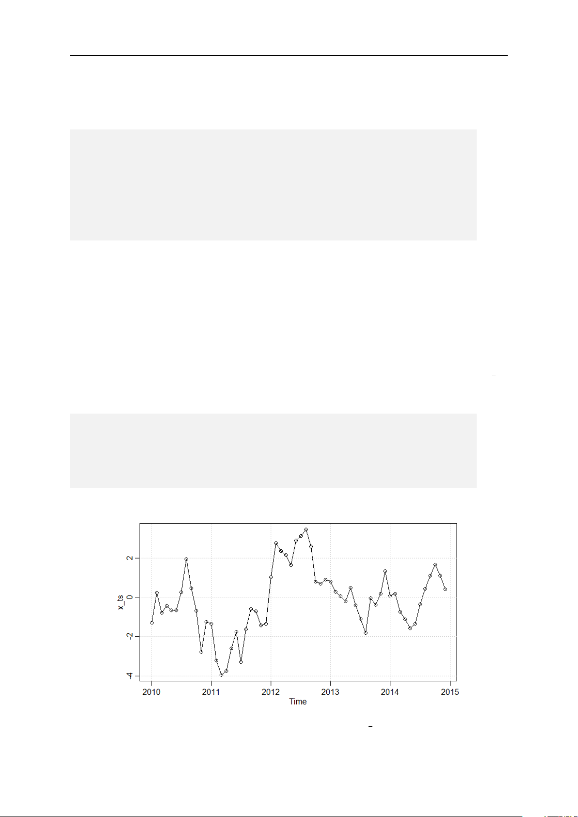
object comes with many useful features. For example, we can generate the plot of x ts
depicted in Figure 1 by simply running the following command:
# p l o t the t i m e s e r i e s
p l o t ( x _ ts , t y p e = " o " )
# add g r i d l i n e s for b e t t e r r e a d a b i l i t y g r i d ()
Figure 1: Plot of the ts() object x ts 6
Introduction to Time Series Econometrics v0.1
We can obtain the data for a specific time window using the function window(). For
example, we can get the observations of the time series x ts from July 2012 onwards by running the following command:
# Get the d a t a f r o m the x _ ts t i m e s e r i e s s t a r t i n g J u l y 2 0 1 2 :
w i n d o w ( x _ ts , s t a r t = c ( 2 0 1 2 , 7 ))
The functions start() and end() return the start and end points of a ts() object.
The function frequency() returns the number of observations per unit of time and the
function time() returns the time index of the ts() object. Throughout this script we
will explore other useful functions specifically designed for ts().4
4The examples and exercises in this script are done with R 4.1.0 and the “astsa” package 1.13 running on Windows 10. 7 CHAPTER ONE BASIC CONCEPTS
In the first chapter of this script, we will introduce basic characteristics of a time series.
Starting with the definition of a time series, we will analyse different examples of time
series datasets. In particular, the concepts of seasonality and trend are introduced. The
relevant chapters in the main references to this script are:
• Chapter 6.1, 6.3, and 8.1 in Forecasting: principles and practice (Hyndman & Athanasopoulos, 2018),
• Chapter 1.1 in Time Series Analysis and Its Applications: With R Examples (Shumway & Stoffer, 2017). 1.1 The nature of time series data
Broadly speaking, a time series represents a collection of data points observed at different
points in time. In its most simple form, a time series is a collection of values indexed in
time order. Most commonly, the time distance between two observations is constant, e.g.
one day or one month. However, this is not always the case. In Table 1.1 we depict two
examples of time series data. The upper panel presents the quarterly earnings per share of 8
Introduction to Time Series Econometrics v0.1
the company Johnson & Johnson. The data is indexed by the year and quarter. Earnings
are a typical example of evenly spaced time series, as the time between two subsequent
observations is constant. The lower panel presents the transactions recorded on the New
York Stock Exchange for the stock of Johnson & Johnson. The data is indexed by the
date, hour, minute, and second. The time between two subsequent transactions is not
constant. For example, there are 14 seconds between the first and second observation,
but only 10 seconds between the second and the third. In this introductory course we
focus exclusively on evenly spaced time series data.
Table 1.1: Examples of time series data
Example of an equally spaced time series: Quarterly earnings Time index
Value: quarterly earnings per share 1960 Q1 0.71$ 1960 Q2 0.63$ 1960 Q3 0.85$ 1960 Q4 0.44$ 1961 Q1 0.61$ .. . . ..
Example of an unevenly spaced time series: Transactions of stocks Time index Value: transaction price 05.01.2001 9:43:46 97.31$ 05.01.2001 9:44:00 97.06$ 05.01.2001 9:44:10 97.00$ 05.01.2001 9:44:18 96.75$ 05.01.2001 9:44:30 96.63$ .. . . ..
Note: The table depicts two example of time series. The upper panel presents
the quarterly earnings per share of the company Johnson & Johnson (source:
“astse” R-package). The data is indexed by the year and quarter. Earnings are a
typical example of evenly spaced time series, as the time between two subsequent
observations is constant. The lower panel presents the transactions recorded on
the New York Stock Exchange for Johnson & Johnson’s stock (source: NYSE
TAQ database). The data is indexed by the date, hour, minute, and second. The
time between two subsequent transaction is not constant.
Time series data appears in many different research fields. In finance, for instance, each
day we observe the closing prices of stocks traded on the market and, as seen in the
previous example, each quarter a publicly traded company publishes its earnings. In 9
Introduction to Time Series Econometrics v0.1
economics, unemployment rates are reported each month. Meteorologists are interested
in the daily recorded temperatures and epidemiologist study the number of new virus
infections over a given time period.
Over the next pages, we will study the plots of some time series. The visual inspection of
these data will uncover some of the typical patterns found in time series data, and over
the remainder of this script, we will learn how to deal with them.
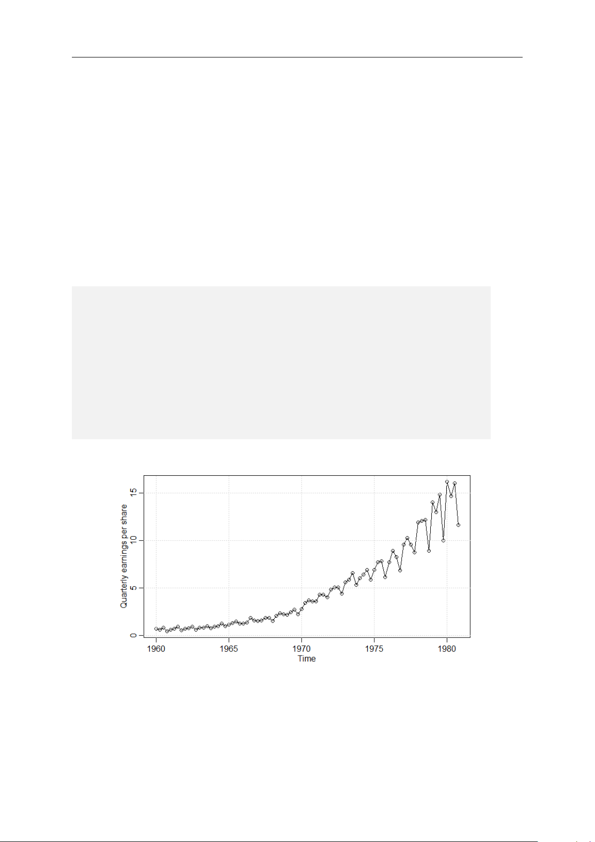
Figure 1.1 plots the time series of Johnson & Johnson’s quarterly earnings per share. The
plot can be generate with the following R commands: l i b r a r y ( a s t s a )
# get the e a r n i n g s of J o h n s o n and J o h n s o n jj _ e a r n i n g s < - jj # p l o t the d a t a
p l o t ( jj _ e a r n i n g s , t y p e = ’ o ’ , m a i n = ’ ’ ,
y l a b = ’ Q u a r t e r l y e a r n i n g s per s h a r e ’ )
# add g r i d l i n e s for b e t t e r r e a d a b i l i t y g r i d ()
Figure 1.1: Plot of the quarterly earnings per share of Johnson & Johnson
From the plot we observe a clear positive trend: over the years the earnings per share
increase considerably. Moreover, compared to the first three quarters, the earnings in the
last quarter are generally smaller. In time series analysis we refer to this pattern as a 10
Introduction to Time Series Econometrics v0.1
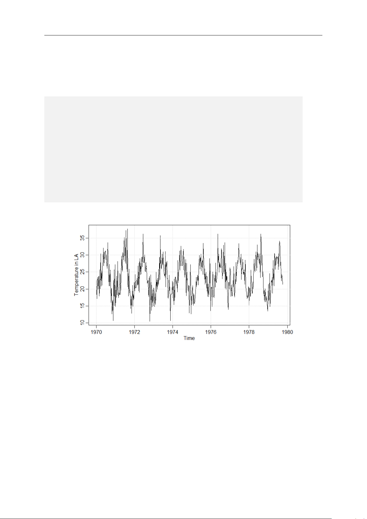
seasonality. Seasonal patterns appear in many different time series. For example, Figure
1.2 shows the weekly temperature measured in L.A. from 1970 to 1980. To obtain the
plot in R you can run the following code:
# get t e m p e r a t u r e d a t a
t e m p _ d a t a < - t e m p r
# t r a n s f o r m F a h r e n h e i t to C e l s i u s
t e m p _ d a t a < - ( t e m p _ data - 3 2 )* 5 / 9 # p l o t the d a t a
p l o t ( t e m p _ data , t y p e = ’ l ’ , m a i n = ’ ’ ,
y l a b = ’ T e m p e r a t u r e in LA ’ )
# add g r i d l i n e s for b e t t e r r e a d a b i l i t y g r i d ()
Figure 1.2: Plot of L.A. temperature
Note that the temperatures are provided in Fahrenheit and I convert them to Celsius
before plotting them. The time series of the temperatures has a clear seasonal pattern:
during the summer the weather is warmer and temperatures are around 30 degrees Cel-
sius, whereas in the winter weeks the temperature drops to roughly 15 degrees Celsius.
Over the short time window between 1970 and 1980 there is no clear trend in the tem- peratures.
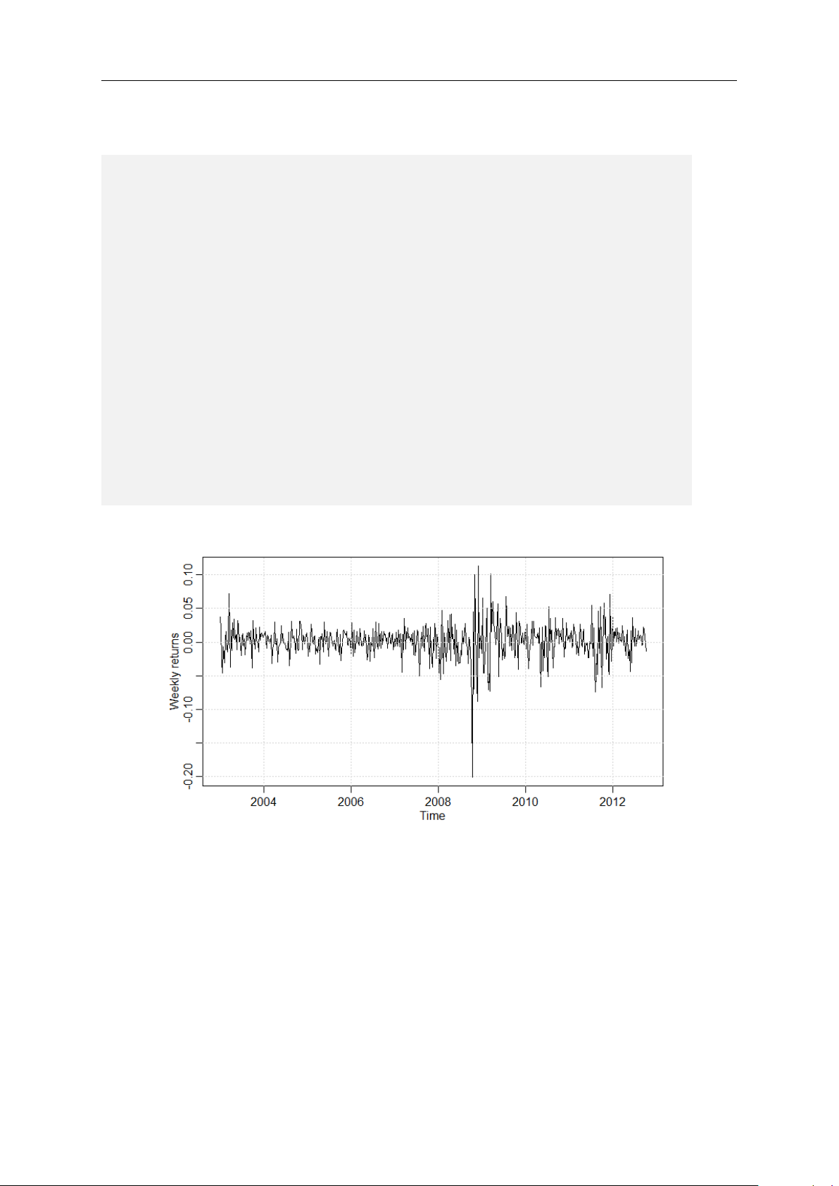
Figure 1.3 depicts the weekly returns of the S&P 500 stock market index from 2003 to 11
Introduction to Time Series Econometrics v0.1
2012. I create the plot by running the following code:
# get w e e k l y r e t u r n s of the SP 5 0 0 i n d e x
sp 5 0 0 _ d a t a < - sp 5 0 0 w
# n o t e t h a t t h i s d a t a c o m e s in the f o r m of an " xts "
# object , w h i c h is a d i f f e r e n t
# c l a s s u s e d in R to h a n d l e t i m e s e r i e s d a t a ;
# we t r a n s f o r m the xts o b j e c t to a ts o b j e c t for
# c o n s i s t e n c y w i t h the o t h e r d a t a
sp 5 0 0 _ d a t a < - ts ( sp 5 0 0 _ data , s t a r t = c ( 2 0 0 3 , 1 ) , f r e q u e n c y = 5 2 ) # p l o t the d a t a
p l o t ( sp 5 0 0 _ data , t y p e = ’ l ’ , m a i n = ’ ’ , y l a b = ’ W e e k l y r e t u r n s ’ )
# add g r i d l i n e s for b e t t e r r e a d a b i l i t y g r i d ()
Figure 1.3: Plot of weekly S&P 500 returns
The weekly return series provided by the “astsa” package comes in the form of an xts
object, which is an extension of the more simple ts data-type used throughout this script.
While you can directly plot xts with the command plot(), for consistency I transform
the weekly returns to a ts object. From a visual inspection, there is no apparent trend
nor seasonal pattern in the weekly returns. We observe however that around the financial
crisis of 2008-2009 the series fluctuates more compared to the other years. This pattern 12
Introduction to Time Series Econometrics v0.1
is known as heterogeneous or time-varying volatility and there are specific approaches to
deal with it. Being more advanced topics that require first a basic understanding of time
series analysis, I will not cover these techniques in this script.
Analyzing the data graphically is a very important part of time series econometrics. It
allows to draw some first conclusions about the relevant properties of the data, such as
seasonal patterns or trends. In Section 1.3 of this chapter I will use the plots of time
series to guide my choice of the appropriate modelling approach. In Chapter 2 I will
introduce useful graphical representations of time series data. 1.2 Notation
Before turning our attention to the statistical properties and approaches used in time
series analysis, it is necessary to introduce some basic notation. In statistical terms, a
time series is a collection of time ordered random variables:
. . . , Yt−2, Yt−1, Yt, Yt+1, Yt+2 . . . (1.1)
where the subscript indicates the time at which the random variable realizes. For example,
when analyzing the quarterly earnings of Johnson & Johnson, Yt represents the (random)
earnings and its index t indicates the year and quarter in which the earnings are published.
Each of these time-ordered random variables has a cumulative distribution function Ft,
which is not necessarily constant over time. Definition 1.1: Time series
A time series in discrete time is a sequence of time-ordered real-valued random variables {Yt : t ∈ Z}.
Often, it will be useful to define how Yt came about. For example, we could assume that 13
Introduction to Time Series Econometrics v0.1
the quarterly earnings are generated by: Yt = Yt−1 + t (1.2)
where t is a standard normally distributed random variable.1 Equation (1.2) can be read
as follows. Let’s assume that t is the first quarter in 1970. Then, the above equation
tells us that the earnings of the first quarter in 1970 are equal to the earnings of the last
quarter in 1969 (i.e. Yt−1) plus some random term which on average is equal zero. We
will explore later in this script whether this is an appropriate model for the quarterly
earnings of Johnson & Johnson.
If we would like to know how the earnings changed from quarter to quarter, we can take
the first difference of Equation (1.2):
∆Yt = Yt − Yt−1 = Yt−1 + t − Yt−1 = t. (1.3)
The first difference is indicated by ∆. In some instances, we might want to take the first
difference more than once. If the first difference of Yt is taken twice, for instance, we
indicate this by ∆∆Yt or ∆2Yt. In other situations, it might be necessary to take the
differences between Yt and Yt−s where s > 1. This type of differences are called seasonal
difference and the notation is ∆sYt = Yt − Yt−s. Definition 1.2: Differencing
First differences in a time series are defined as: ∆Yt = Yt − Yt−1 and for k > 1 ∆kYt = ∆k−1∆Yt.
Seasonal differences are defined as: ∆sYt = Yt − Yt−s.
1Recall that a standard normally distributed random variable has zero mean and unit standard deviation. 14
Introduction to Time Series Econometrics v0.1 1.3
Decomposition of a time series: trend and sea- sonality
In the first part of this chapter, I presented different examples of time series. A visual
inspection thereof highlighted some important patterns that are found in many time
series. In particular, a time series may have one or more of the following properties:
• Seasonal pattern: the time series is affected by a pattern reoccurring at fixed and
known frequency. Seasonal factors can be related, for example, to the time, the
day, the week, the month, or the season.
• Trend: represents a long-term increase or decrease in the time series. It does not
have to be linear and is allowed to change direction over time.
• Cycle: the data exhibit rises and falls that are not of a fixed frequency. For example,
business cycles do not have fixed frequency, and are therefore not a seasonality.
When analyzing a time series, we usually consider trend and cycles jointly. In other
words, we distinguish only between seasonal patterns and trend-cycle patterns. In more
detail, a time series Yt is usually assumed to have the following structure: Yt = Tt + St + Xt (1.4)
where Tt is the trend-cycle component, St is the seasonal component, and Xt is a random
component (often called the remainder term). It is common to treat Tt and St as deter-
ministic functions, i.e. once we know their functional form we can perfectly predict them.
In contrast, Xt is a random variable that is not perfectly predictable. For example, recall
the example of Johnson & Johnson’s quarterly earnings. The visual inspection of this
time series unveiled a positive trend (Tt) and a seasonal pattern (St). The seasonal and
the random remainder components are on average equal to zero. In general, in time series
econometrics the goal is to appropriately model each of the three components. 15
Introduction to Time Series Econometrics v0.1
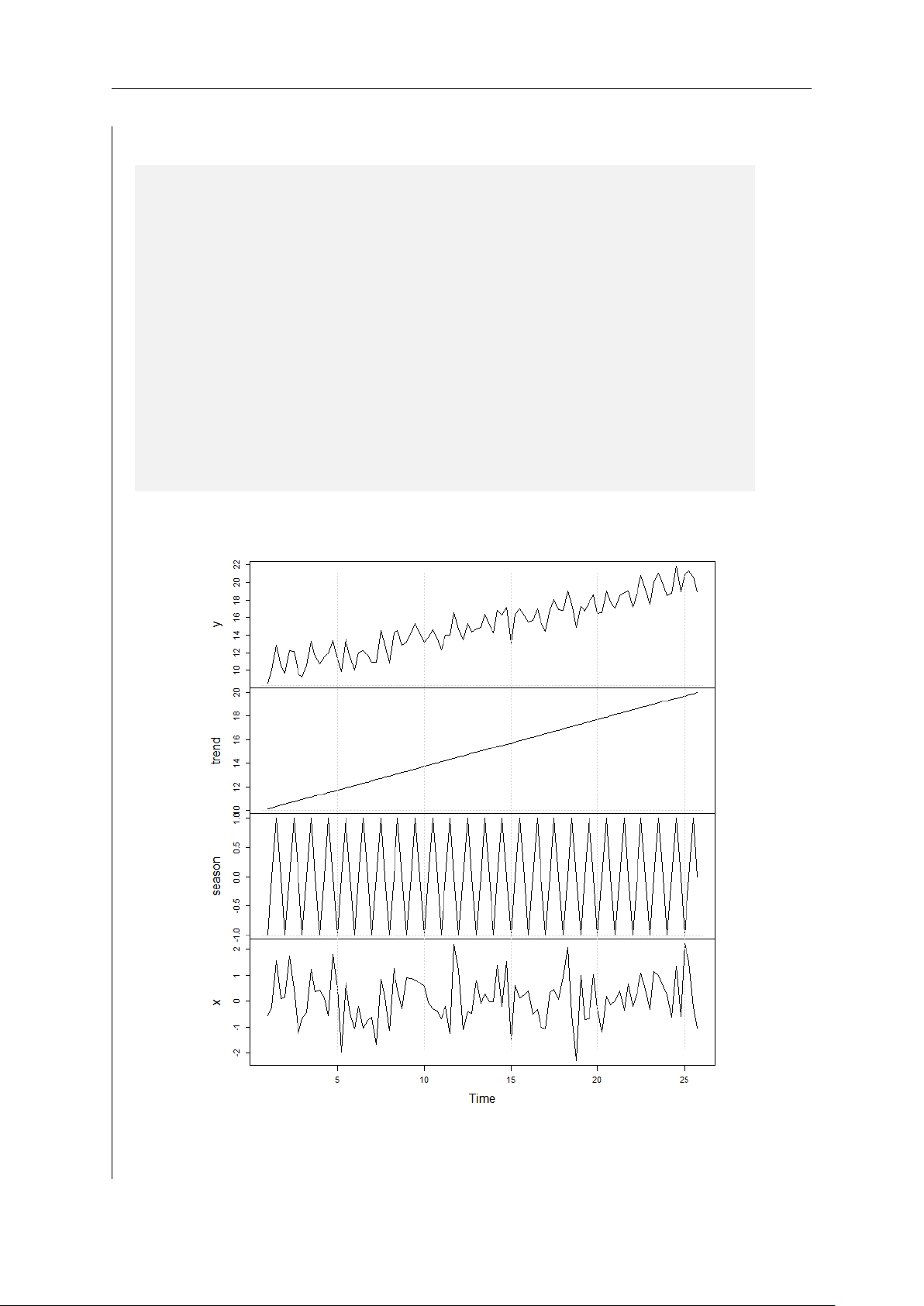
Example 1.1: Time series components
To get a better intuition of the above decomposition of a time series, let’s have a look
at an artificial example. Let the time series Yt have the linear trend Tt = 10 + 0.1 · t,
and a seasonal pattern whose first four observations are: S1 = −1, S2 = 0, S3 = 1, S4 = 0
and repeat every fourth observations, i.e. St = St+4. In other words, S5 will equal
-1, S6 will equal 0, etc. For simplicity, let the random component be a standard
normally distributed random variable. Figure 1.4 plots the time series Yt and its three
components. The figure shows in the top panel, the time series Yt which exhibits a
positive time trend and a seasonal pattern. The second and third panel of Figure
1.4 show these two components: a linear positive trend and a seasonal pattern. The
bottom panel of the figure plots the random component Xt. You can reproduce this
example by running the following R code:
# G e n e r a t e the e x a m p l e of a t i m e s e r i e s d e c o m p o s i t i o n
# To r e p r o d u c e the results , set the s e e d set . s e e d ( 1 2 3 )
# D e f i n e the n u m b e r of o b s e r v a t i o n s in the t i m e s e r i e s n < - 1 0 0
# C r e a t e the t r e n d c o m p o n e n t
t r e n d < - 1 0 + 0 . 1 * 1 : n
# C r e a t e the s e a s o n a l c o m p o n e n t :
s e a s o n < - rep ( c ( - 1 , 0 , 1 , 0 ) , n / 4 )
# G e n e r a t e the r a n d o m c o m p o n e n t
x < - r n o r m ( n , m e a n = 0 , sd = 1 )
# D e f i n e the t i m e s e r i e s
y < - t r e n d + s e a s o n + x
Note that in R we produce the seasonal component by repeating the vector of the
seasonal pattern. The final time series y is obtained by simply summing up the
components. We can then convert the vectors of y, trend, season, and x to ts 16
Introduction to Time Series Econometrics v0.1 objects and plot the results:
# L e t s c o n v e r t all c o m p o n e n t s i n t o ts - o j e c t s and m e r g e t h e m
y < - ts ( y , s t a r t = c ( 1 , 1 ) , f r e q u e n c y = 4 )
t r e n d < - ts ( trend , s t a r t = c ( 1 , 1 ) , f r e q u e n c y = 4 )
s e a s o n < - ts ( season , s t a r t = c ( 1 , 1 ) , f r e q u e n c y = 4 )
x < - ts ( x , s t a r t = c ( 1 , 1 ) , f r e q u e n c y = 4 )
# c o m b i n e the t i m e s e r i e s y and its c o m p o n e n t s # in one o b j e c t :
ts _ c o m p o n e n t s < - ts . u n i o n ( y , trend , season , x )
# p l o t the t i m e s e r i e s and its c o m p o n e n t s
p l o t ( ts _ c o m p o n e n t s , t y p e = " l " , m a i n = " " ) g r i d ()
Figure 1.4: Plot of the time series Yt and its components 17
Introduction to Time Series Econometrics v0.1
An alternative specification of the decomposition of a time series is the following: Yt = Tt · St · Xt. (1.5)
This decomposition is usually referred to as multiplicative decomposition, whereas Equa-
tion 1.4 is referred to as additive decomposition. A simple guideline to choose which
decomposition is most appropriate is as follows:
• Additive decomposition: the seasonal variation or the fluctuation around the trend-
cycle component do not vary with the level of the time series.
• Multiplicative decomposition: the seasonal variation and/or the fluctuation around
the time-cycle are proportional to the level of the time series.
While there are techniques to directly work with the multiplicative decomposition, in this
course we will transform these time series by taking the natural logarithm. In fact, if we
take the natural logarithm on both sides of Equation (1.5) we obtain: log(Yt) = log(Tt · St · Xt) = log(Tt) + log(St) + log(Xt) (1.6)
and the transformed time series log(Yt) has an additive decomposition. In other words,
when we suspect that the time series Yt has a multiplicative decomposition, we transform it and work with log(Yt). 18
Introduction to Time Series Econometrics v0.1
Definition 1.3: Decomposition of a time series
A time series Yt has an additive decomposition when it can be defined as: Yt = Tt + St + Xt T T 1 X 1 X with St = 0 and Xt = 0 T T t=1 t=1
where Tt is a deterministic trend-cycle component, St is a deterministic seasonal
component and Xt is a random component. The time series has instead a multi-
plicative decomposition, if the seasonal variation and/or the fluctuation around the
time-cycle are proportional to the level of the time series: Yt = Tt · St · Xt 1 1 T ! T T ! T Y Y with St = 1 and Xt = 1 t=1 t=1 1.4
The goal of time series analysis
The general goal of time series analysis is to make inference about a time series Yt. For
example, we might be interested in forecasting next year’s sales of Amazon. Or, we would
like to quantify the impact of seasonalities of the earnings of Johnson & Johnson. All
these tasks involve the definition and estimation of a probabilistic model for the time series.
The analysis of time series data proceeds roughly as follows. First, we visually inspect
the data. We try to identify the properties of the time series to guide our choice of an
appropriate model. Second, we define a model for the trend and seasonal component.
Third, we estimate the trend and the seasonal component and determine the random remainder component: b Xt = Yt − b Tt − b
St, where the “hat” highlights the fact that we
have estimated these components. Fourth, we analyze the remainder term. In some cases, b
Xt is an independent and identically distributed random variable (i.i.d.), in which case 19