Solutions manual - Quantitative method for Finance
Tài liệu học tập môn Finance - Banking (MFBO19) tại Trường Đại học Quốc tế, Đại học Quốc gia Thành phố Hồ Chí Minh. Tài liệu gồm 66 trang giúp bạn ôn tập hiệu quả và đạt điểm cao! Mời bạn đọc đón xem!
Môn: Finance - Banking (MFBO19) 10 tài liệu
Trường: Trường Đại học Quốc tế, Đại học Quốc gia Thành phố Hồ Chí Minh 1.9 K tài liệu
Tác giả:


Preview text:
lOMoARcPSD|359 747 69 Solutions Manual to
AN INTRODUCTION TO MATHEMATICAL
FINANCE: OPTIONS AND OTHER TOPICS Sheldon M. Ross 1 1.1 1.2 1.3 1.4 1.5
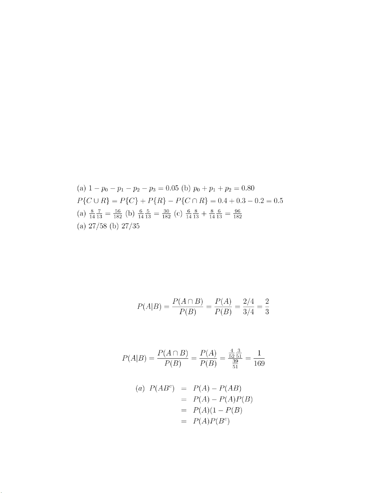
1. The probability that their child will develop cystic fibrosis is the probability thatthe
child receives a CF gene from each of his parents, which is 1/4.
2. Given that his sibling died of the disease, each of the parents much have exactlyone
CF gene. Let A denote the event that he possesses one CF gene and B that he does
not have the disease (since he is 30 years old). Then
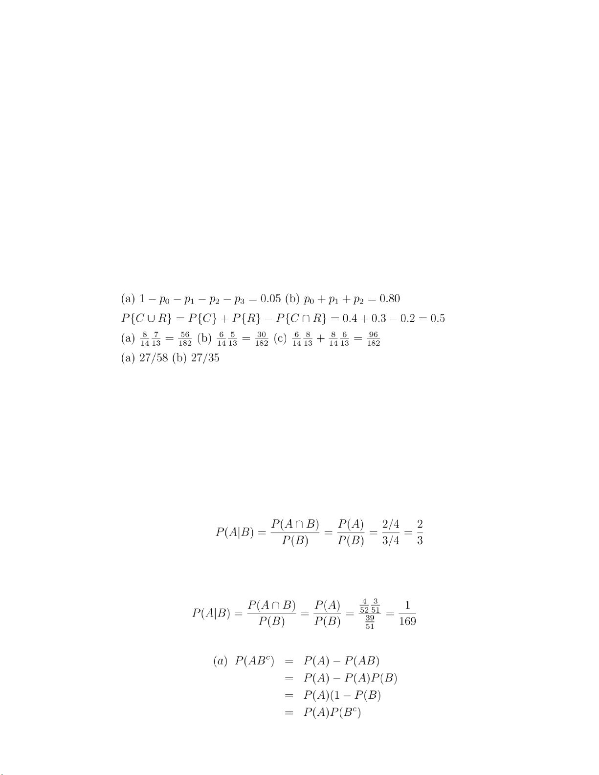
1.6 Let A be the event that they are both aces and B the event they are of different suits. Then 1.7 lOMoARcPSD|359 747 69
Part (b) follows from part (a) since from (a) A and Bc are independent, implying from (a)
that so are Ac and Bc.
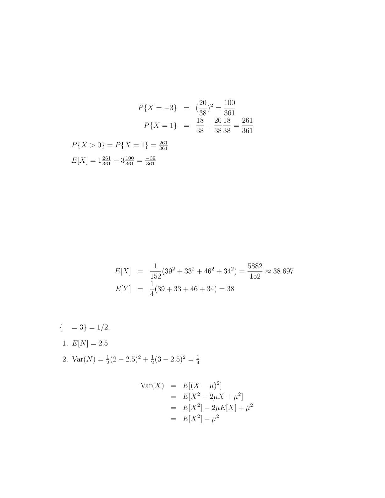
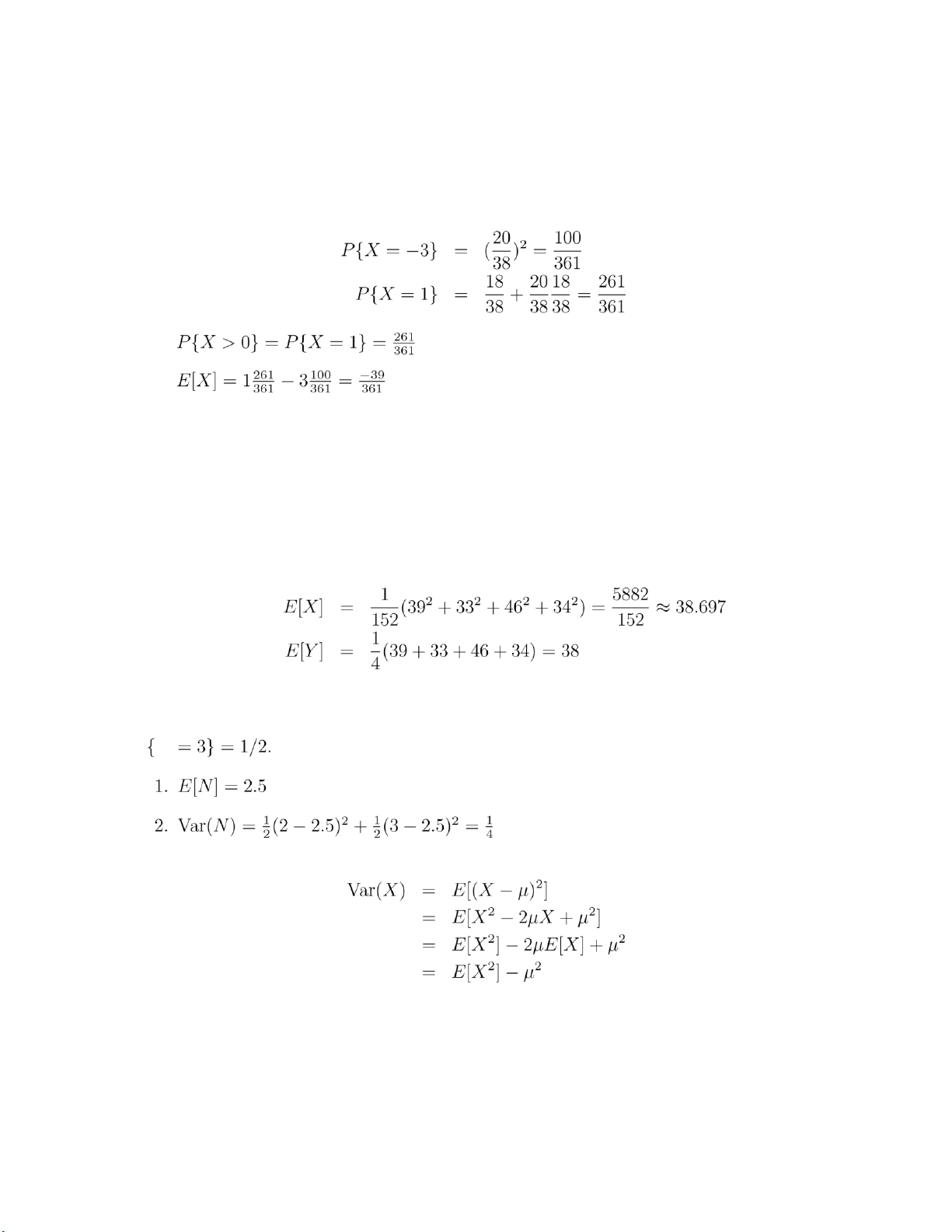
1.8 If the gambler loses both the bets, then X = −3. If he wins the first bet, or loses the
first bet and wins the second bet, X = 1. Therefore, 1. 2. 1.9 2
1. E[X] is larger since a bus with more students is more likely to be chosen than a bus with less students. 2.
1.10 Let N denote the number of sets played. Then it is clear that P{N = 2} = P N
1.11 Let µ = E[X].
1.12 Let F be her fee if she takes the fixed amount and X when she takes the contingency amount. lOMoARcPSD|359 747 69
E[F] = 5,000, SD(F) = 0
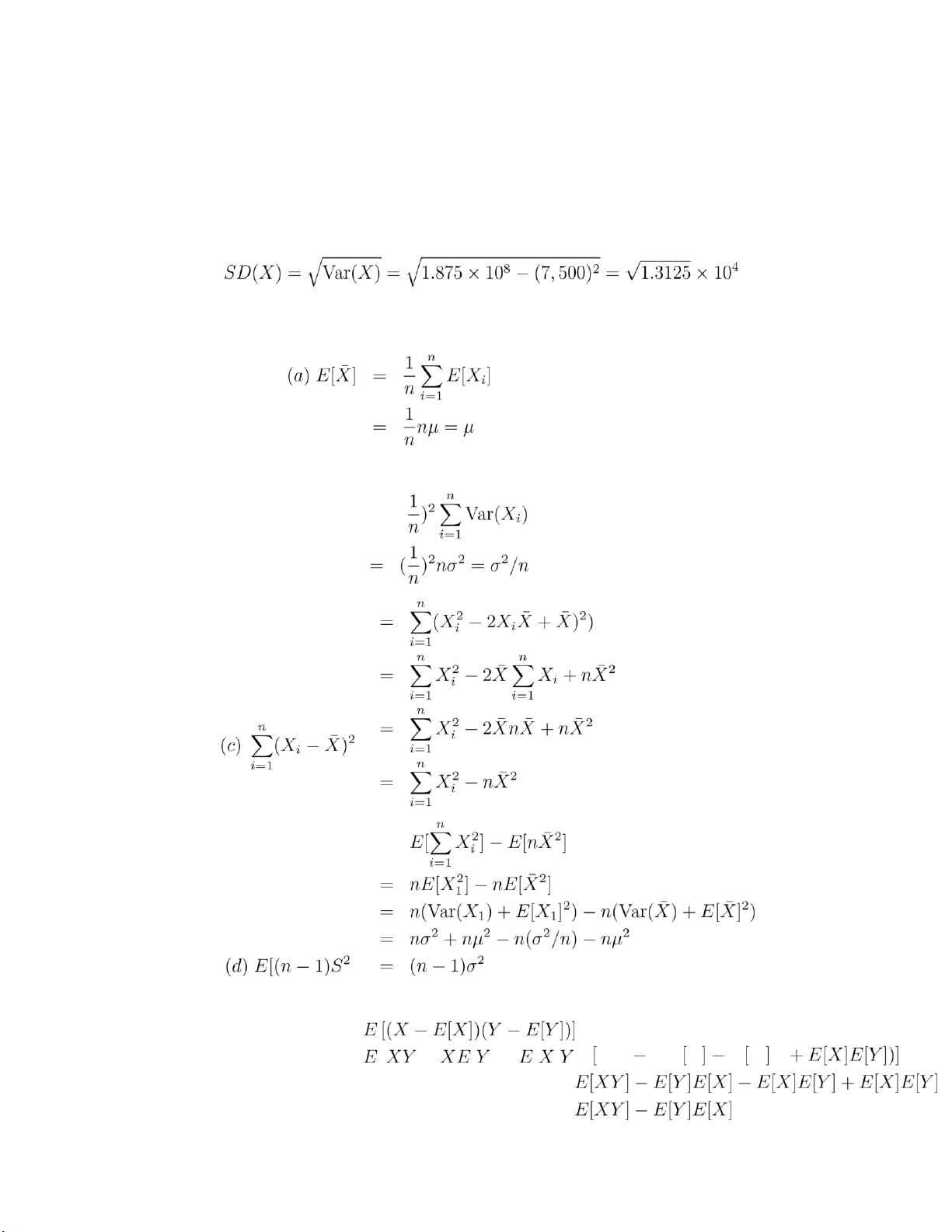
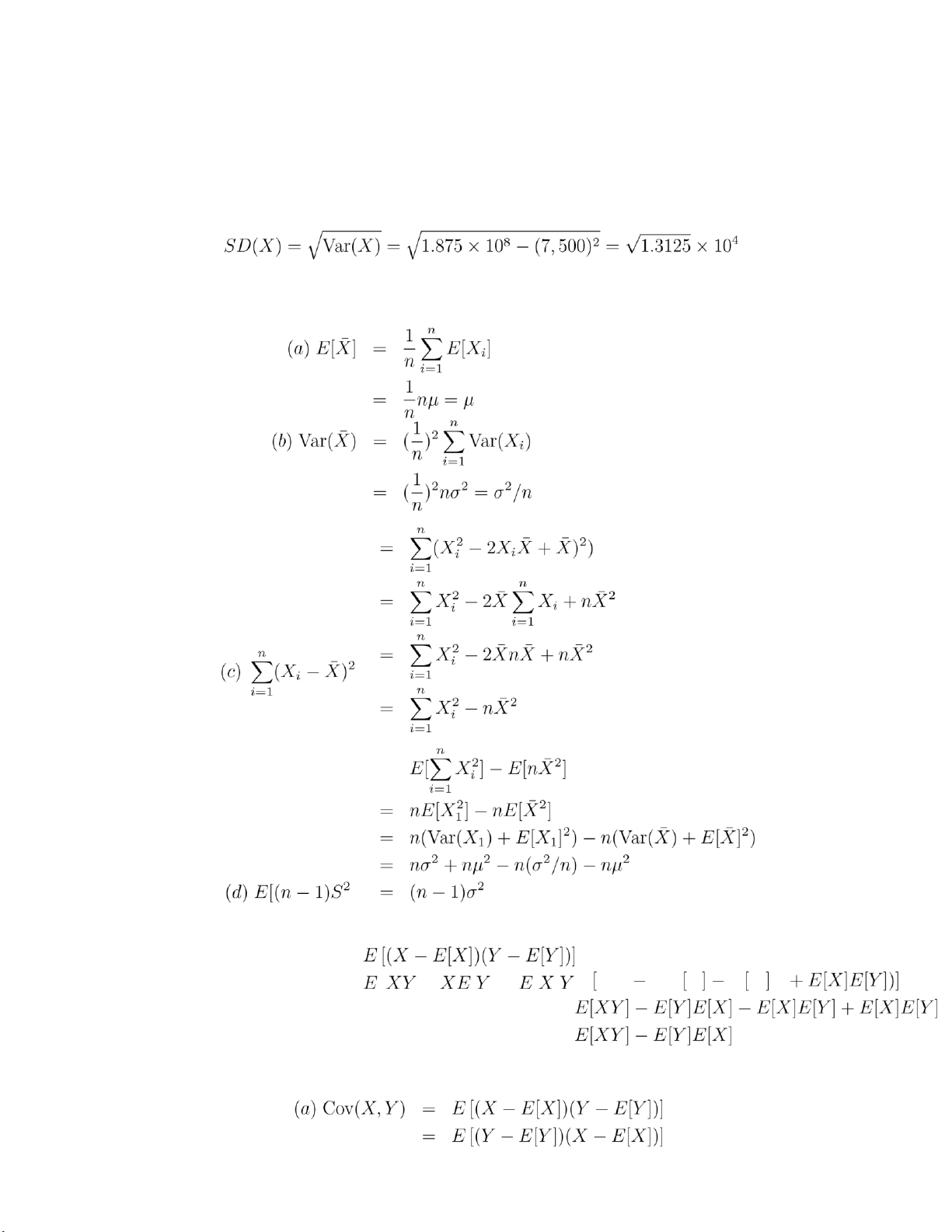
E[X] = 25,000(.3) + 0(.7) = 7,500
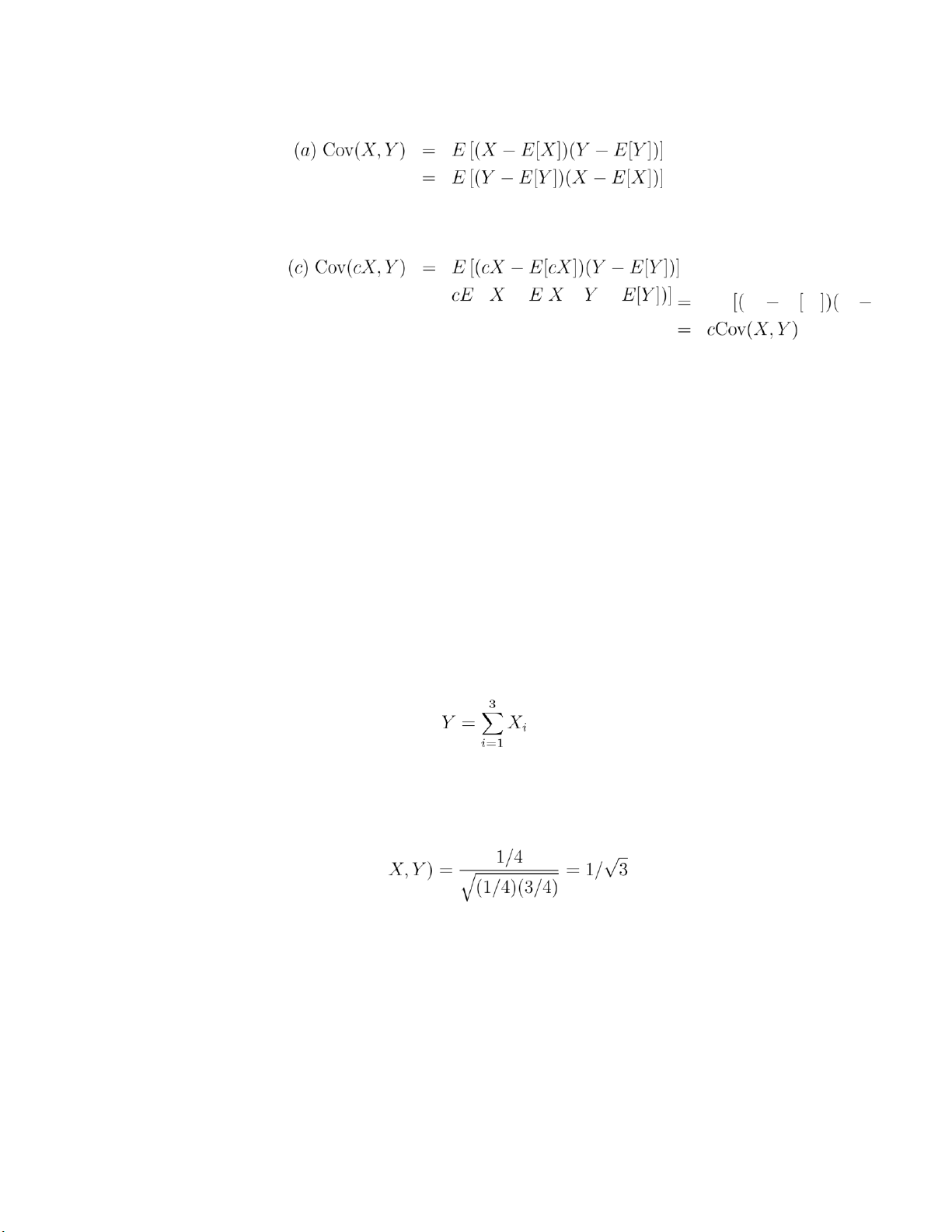
E[X2] = (25,000)2(.3) + 0(.7) = 1.875 × 10⁸ Therefore, 1.13 3 (b) Var(X¯) = ( ] = 1.14 Cov(X,Y ) = = = = lOMoARcPSD|359 747 69 1.15 (b) Cov(X,X) =
E[(X − E[X])2] = Var(X) (d) Cov(c,Y ) =
E [(c − E[c])(Y − E[Y ])] = 0 4 1.16
Cov(aU + bV,cU + dV ) =
Cov(aU,cU + dV ) + Cov(bV,cU + dV ) =
Cov(aU,cU) + Cov(aU,dV ) + Cov(bV,cU) + Cov(bV,dV )
= ac(1) + ad(0) + bc(0) + bd(1) = ac + bd
1.17 With c(i,j) = Cov(Xi,Xj)
(a) c(1,3) + c(1,4) + c(2,3) + c(2,4) = 21
(b) 2 + 3 + 4 + 4 + 6 + 8 + 6 + 9 + 12 = 54 1.17
Let Xi be the amount it goes up in period i. Then and
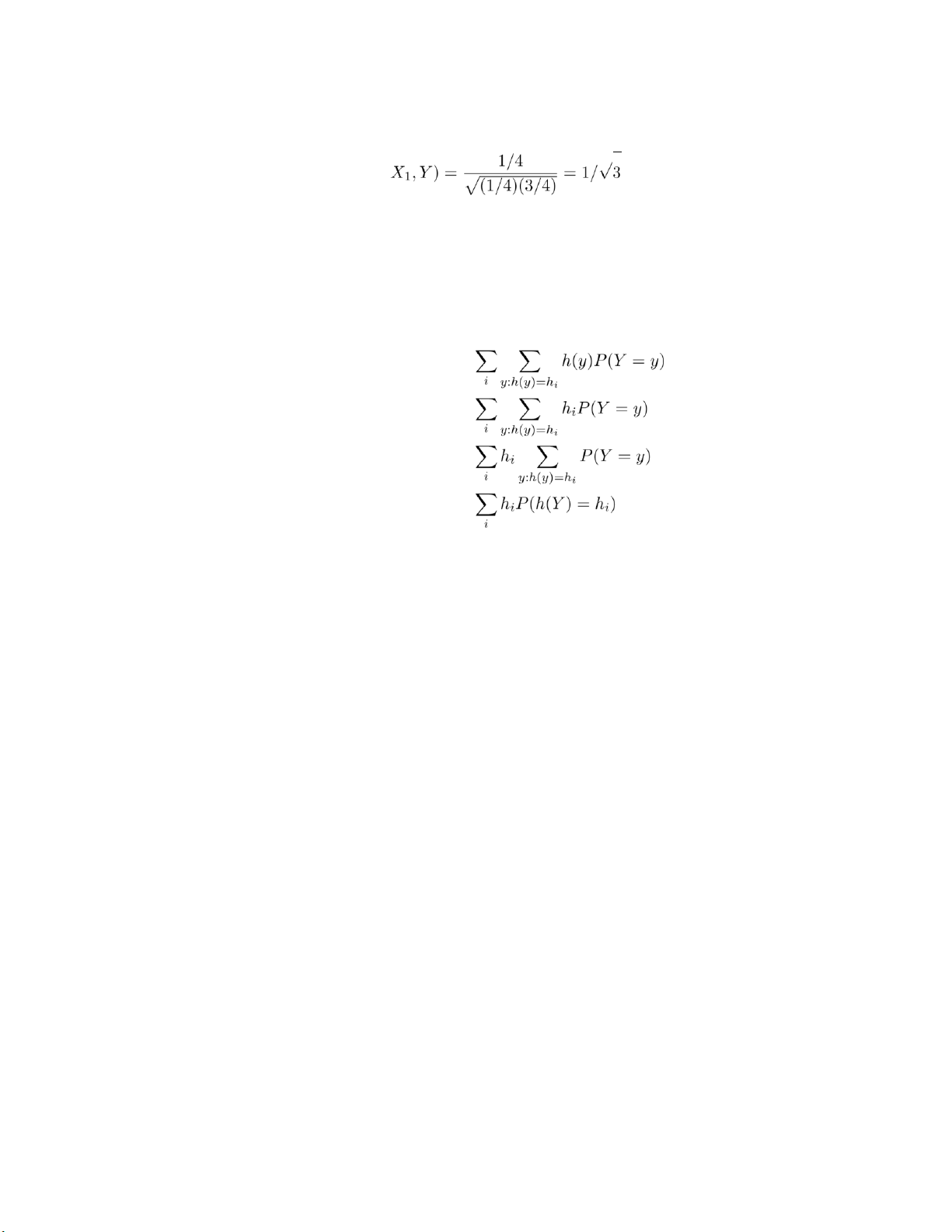
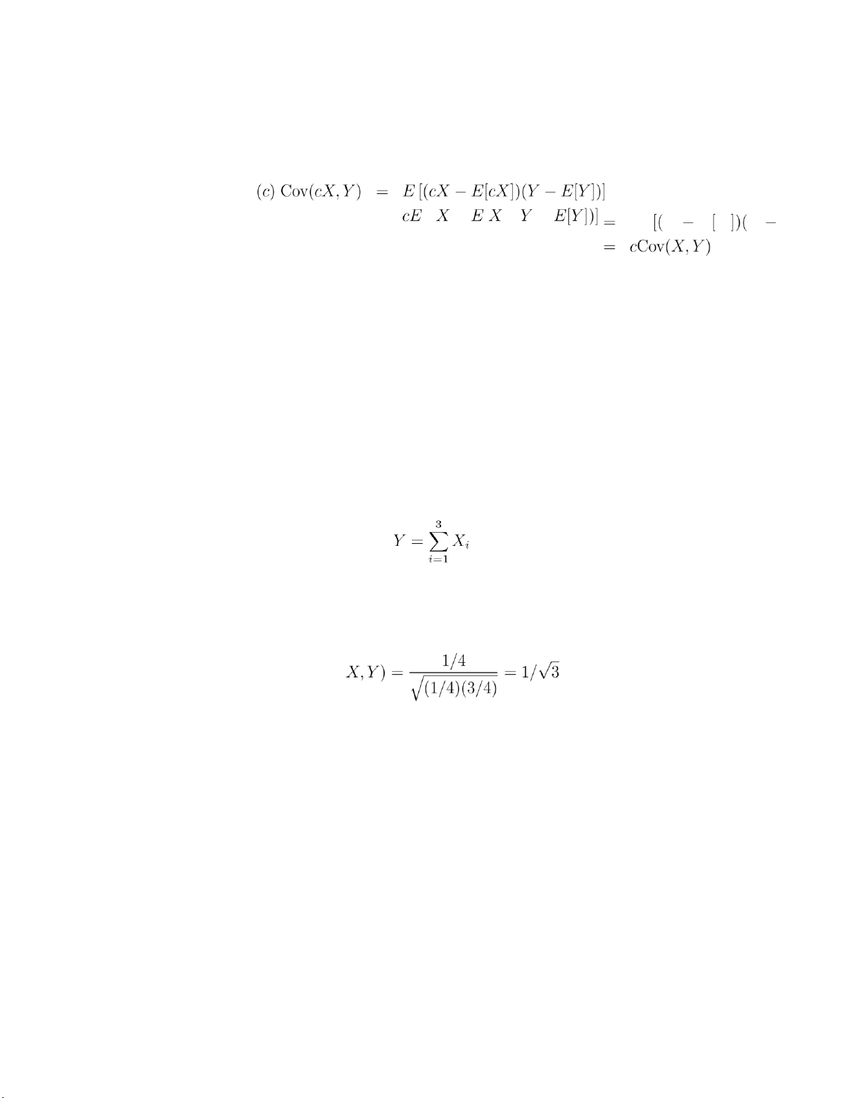
Cov(X1,Y ) = Cov(X1,X1) = Var(X1) = 1/4 Therefore, Corr( 1.18
No, since for such a pair Corr(X,Y ) = 2, and correlations are always between −1 and 1.
1.18 Let Xi be the amount it goes up in period i. Then 3 Y = XXi i=1 and
Cov(X1,Y ) = Cov(X1,X1) = Var(X1) = 1/4 lOMoARcPSD|359 747 69 Therefore, Corr(
1.19 No, since for such a pair Corr(X,Y ) = 2 and correlations are always between −1 and 1. 1.20
h(y)P(Y = y) = X y = = =
1.21 P(X = i) = F(i) − F(i − 1) 2 5 2.1
1. P(Z < −.66) = P(Z > .66) = 1 − P(Z < .66) = 1 − Φ(.66) = 1 − .7454 = .2546 2. lOMoARcPSD|359 747 69
P(|Z| < 1.64) =
P(Z < 1.64) − P(Z < −1.64) =
P(Z < 1.64) − [1 − P(Z < 1.64)]
= 2Φ(1.64) − 1 = 2 × .9495 − 1 = .8990
3. P(|Z| > 2.20) = 2P(Z > 2.20) = 2[1 − P(Z < 2.20)] = 2(1 − .9861) = .0278 2.2 x = 2 2.3
P(|Z| > x) = P(Z > x or Z < −x) = P(Z > x) + P(Z < −x) = 2P(Z > x)
where the last equality comes from the fact that Z is symmetric. 2.4 a = 2µ, b = −1.
Cov(X,Y ) = −Var(X) = −σ2 2.5
(a) 127.7 ± 19.2
(b) 127.7 ± (1.96)(19.2)
(c) 127.7 ± 57.6
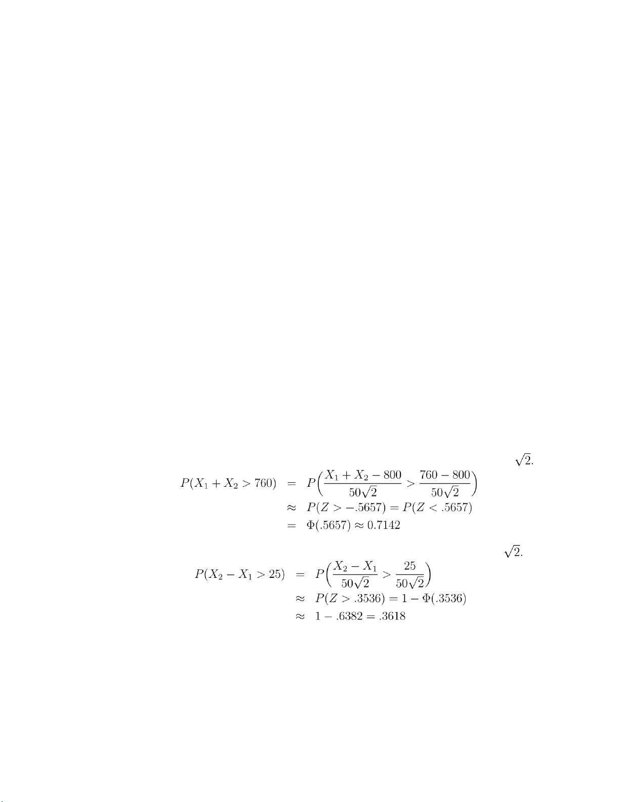
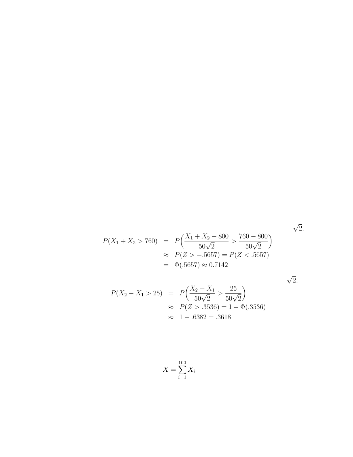
2.6 Let X1 and X2 denote the life of the first and the second battery respectively. It is
given that X1 and X2 are both normal random variables with mean 400 and standard
deviation 50. Let Z denote a standard normal random variable.
1. X1 +X2 is a normal random variable with mean 800 and standard deviation 50
2. X2 − X1 is a normal random variable with mean 0 and standard deviation 50 6
3. P(|X1 − X2| > 25) = 2P(X2 − X1 > 25) ≈ .7236
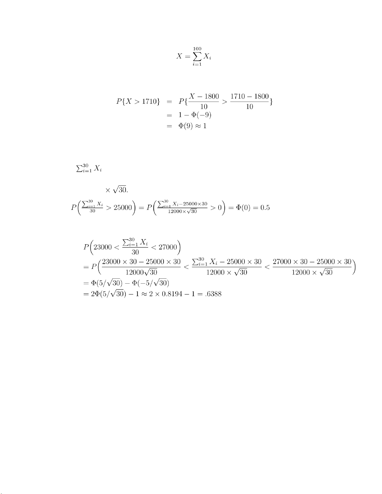
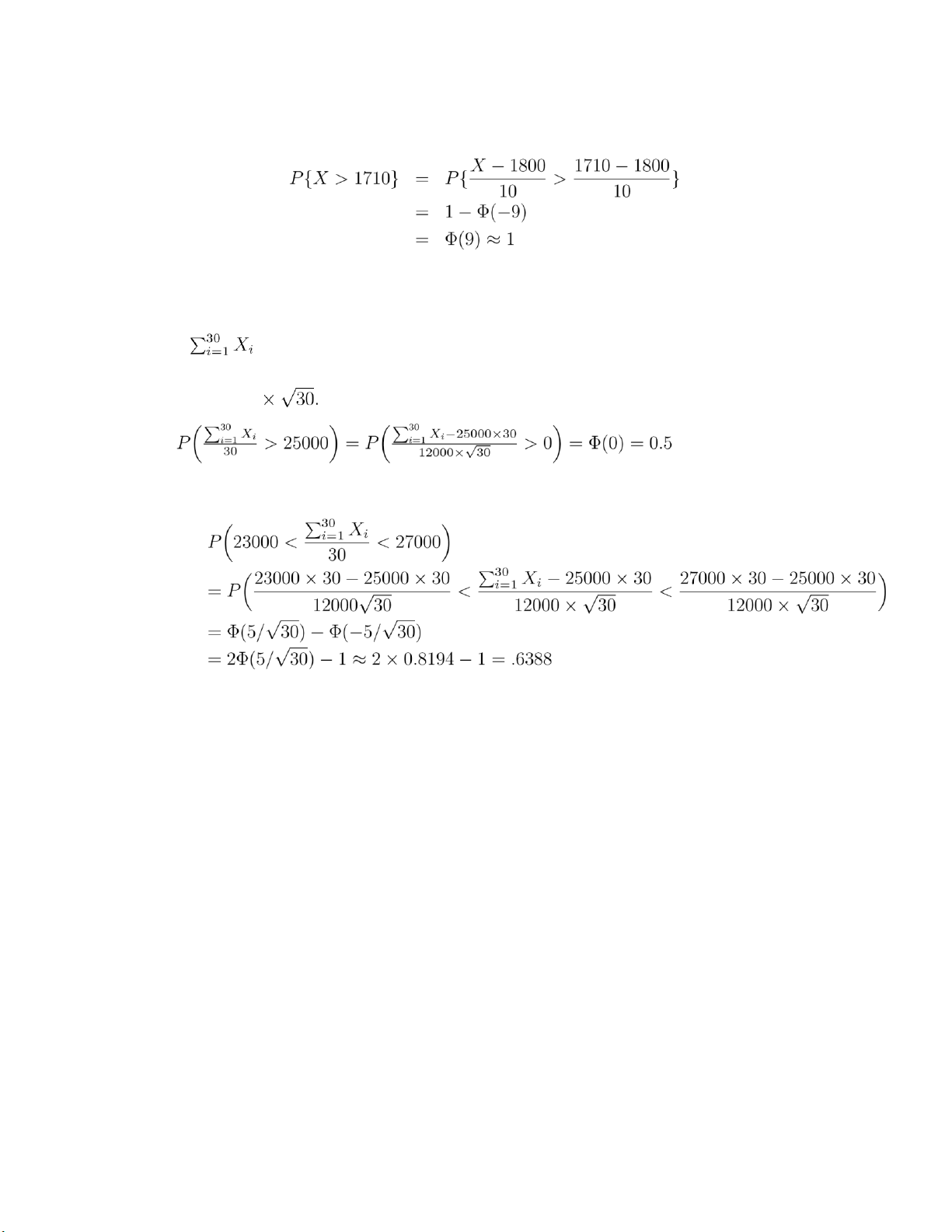
2.7 Let Xi be the time the that it takes to develop the ith print. Then, the time that
it takes to develop 100 prints, call it X, can be expressed as lOMoARcPSD|359 747 69
It follows from the central limit theorem that X approximately has a normal distribution
with mean 1800 and standard deviation 10. Therefore,
The probability for part (b) is 0
2.8 Let Xi be the mileage for person i, i = 1,...,30. From central limit theorem,
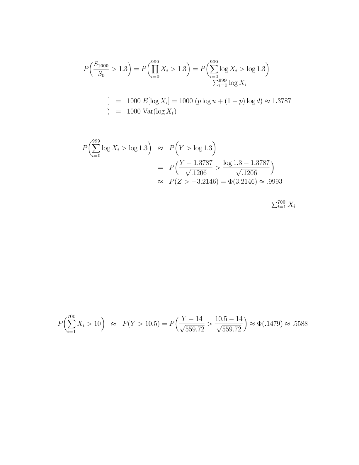
is approximately a normal random variable with mean 25000× 30 and standard deviation 12000 1. 2.
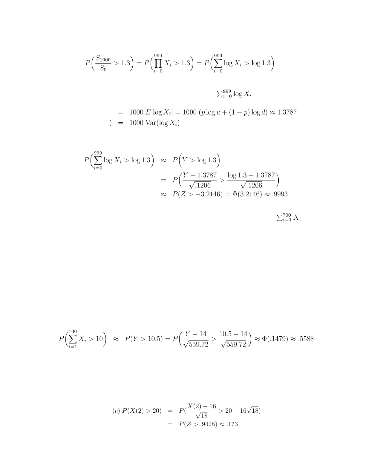
2.9 Let Si be the price of stock in time period i. Then Si+1 = SiXi where the random
variable Xi is defined as
u ,with probability p
d ,with probability 1 p Xi = ( − lOMoARcPSD|359 747 69 Then 7
We can use the central limit theorem to approximate with a normal random
variable Y with the same mean and variance. E[Y ] = Var(Y ) =
= 1000 (p(logu)2 + (1 − p)(logd)2 − .00137872) ≈ 0.1206 Therefore
where Z stands for a standard normal random variable.
2.10 Let Xi be the movement in period i. Then we can approximate with a
normal random variable Y with the same mean and variance 700 · E[Y ] =
EXXi¸ = 700(−.39 + .41) = 14 i=1 700 µ Var(Y ) =
VarXXi¶ = 700(.39 × 1.022
+ .20 × .022 + .41
× .982) = 559.72 i=1 Therefore,
3.1 This follows since −X(t + y) − (−X(y)) = −(X(t + y) − X(y)) is the negative of a normal
with mean µt and variance σ2t, and so has mean −µt and variance σ2t. 3.2 (a) 16; (b) 18 lOMoARcPSD|359 747 69
where Z is a standard normal. 3.3
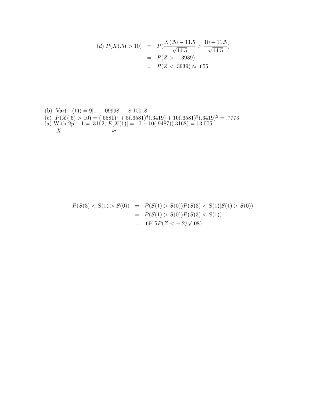
3.4 (a) With W being normal with mean .1 and variance .04,
P(S(1) > S(0)) = P(eW > 1) = P(W > 0) = P(Z > −.1/.2) = P(Z < .5) = .6915 (b) (.6915)2 (c)
3.6 S(t)/s is distributed as eW , where W is normal with mean µt and variance tσ2. Hence,
E[S(t)] = sE[eW ] = seµt+tσ2/2 and
E[S2(t)] = s2E[e2W ] = s2e2µt+2tσ2 3 Hence,
Var(S(t)) = s2e2µt+2tσ2 − s2e2µt+tσ2 = s2e2µt+tσ2(etσ2 − 1)
3.7 This follows directly from the formula for P(Ty ≤ t) given in the text, upon using that limx→∞
Φ(¯ x) = 0 and limx→∞ Φ(¯ −x) = 1. Hence, when µ < 0, lOMoARcPSD|359 747 69
P(M > y) = P(Ty < ∞) = e2yµ/σ2, y > 0
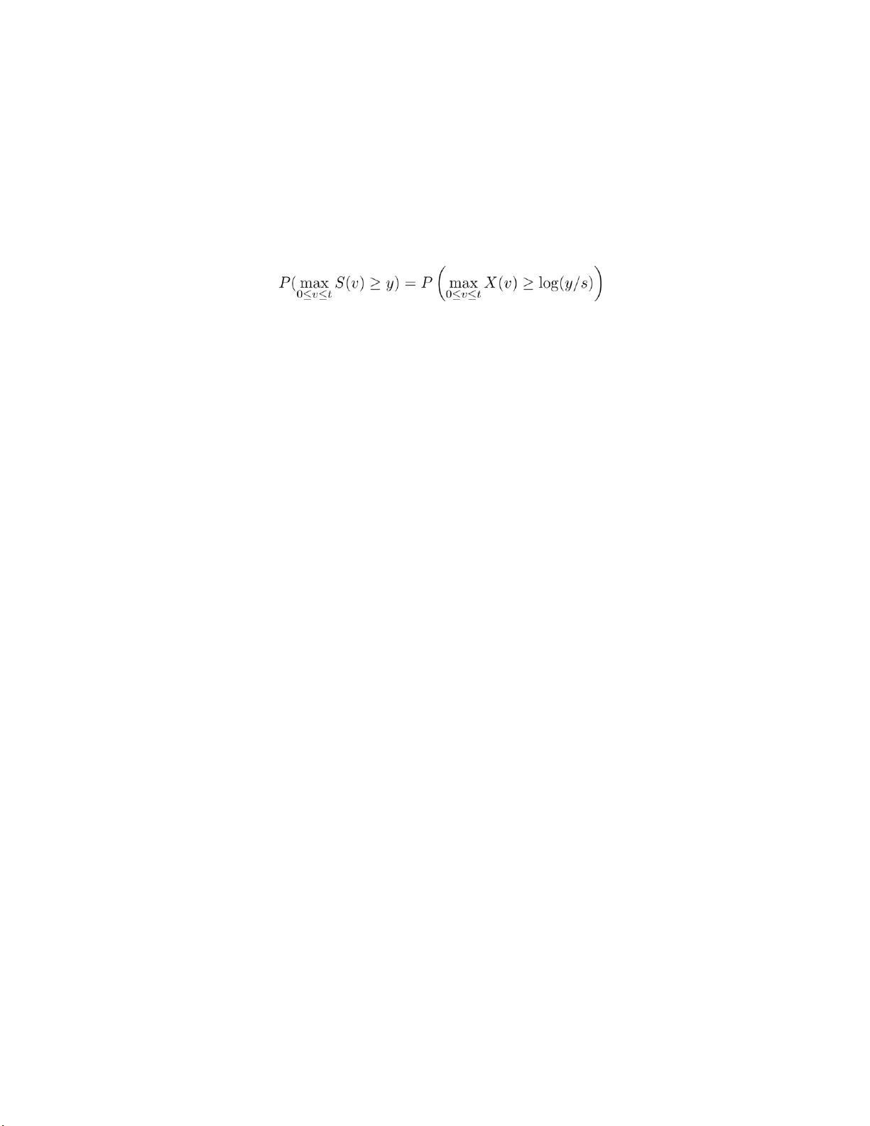
3.8 Using the representation that S(t) = seX(t), where X(t),t ≥ 0 is Brownian motion with X(0) = 0, gives
Now use Corollary 1, setting t = log(y/s).
3.9 The desired probability is P (M(t) < log(1.2)) where M(t) is the maximum by time t of a
Brownian motion having µ = .1,σ = .3 and X(0) = 0. Now, apply Corollary 1. 4 9 4.1
(a) re = (1 + 0.1/2)2 − 1 = 0.1025
(b) re = (1 + 0.1/4)4 − 1 ≈ 0.1038 lOMoARcPSD|359 747 69
(c) re = e0.1 − 1 ≈ 0.1052
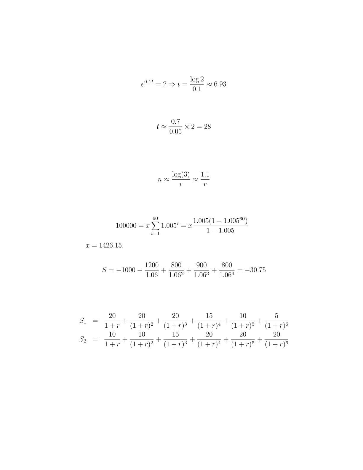
4.2 Suppose it takes t years to double, then
4.3 Suppose it takes t years to quadruple, then we can solve t from 1.05t = 4. We
can also use the doulbing rule to approximate t, which gives
If the interest is 4%, then it is approximately 0.7/0.04 × 2 = 35 years.
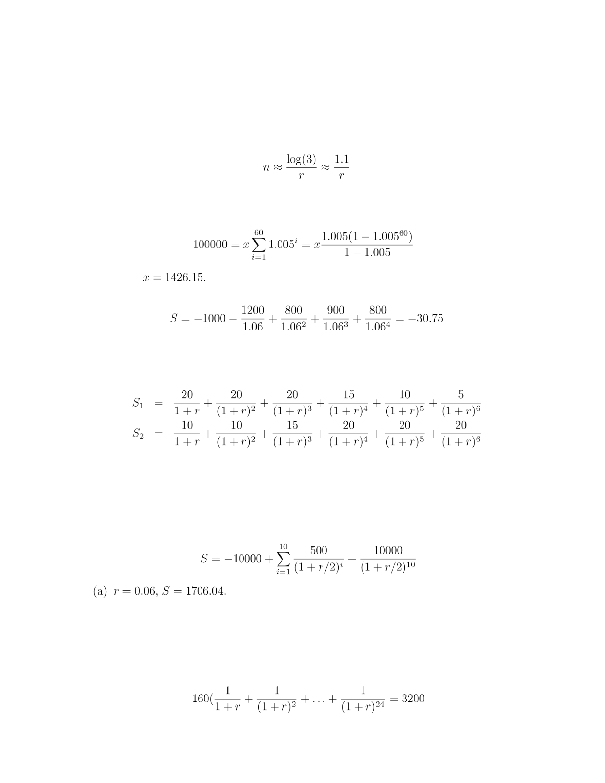
4.4 Using that er ≈ 1+r, when r is small, we see that if (1+r)n = 3 then enr ≈ 3. Thus,
4.5 Suppose you need to invest x at the beginning of each of the next 60 months
to have a value of $100,000 at the end of 60 months, then Solve to get
4.6 Let’s compute the present value, denoted by S, of this cash flow.
Since it is negative, it is not worth investing.
4.7 (15 pts) Let the present value of the first cash flow sequence be S1 and that
of the second cash flow sequence be S2. Then 10
(a) r = 0.03, S1 = 82.71,S2 = 84.63. The second one is preferable. (b) r =
0.05, S1 = 78.37,S2 = 78.60. The second one is preferable.
(c) r = 0.1, S1 = 69.01,S2 = 65.99. The first one is preferable.
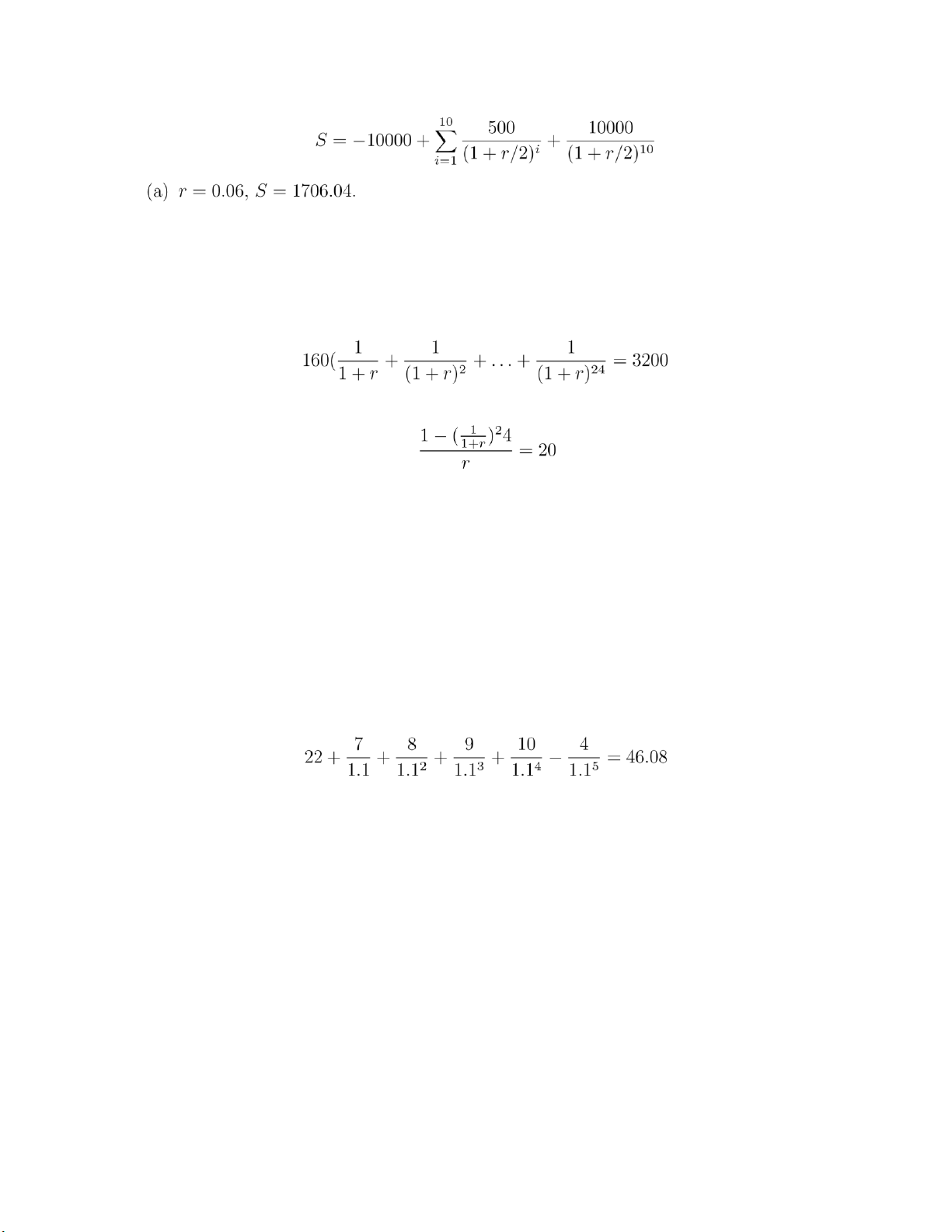
4.8 (15 pts) Let S denote the present value, then lOMoARcPSD|359 747 69
(b) r = 0.10, S = 0.
(c) r = 0.12, S = −736.01.
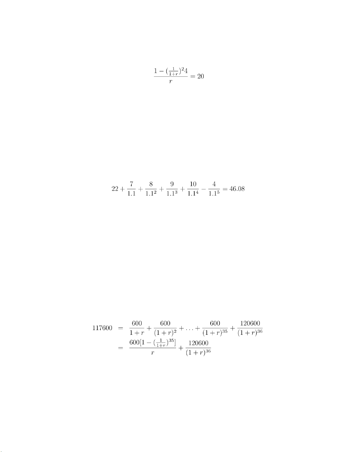
4.9 The effective interest rate, call it r, is that value for which which reduces to
Solution by trial and error shows that r ≈ .015. That is, the effective interest rate is 1.5 percent per month. 4.11
The cost-flow sequences are as follows
buy at beginning of year 1: 22 7 8 9 10 -4 buy at
beginning of year 2: 9 25 7 8 9 -9 buy at beginning of year 3: 9 11 28 7 8 -14
buy at beginning of year 4: 9 11 13 31 7 -19
With the yearly interest rate 10%, the present value of the first cost-flow sequence is
Similarly, the prevent values of the other three cost-flow sequences can be determined,
and the four present values are
46.08, 44.08, 44.17, 46.02
Therefore, the company should purchase a new machine one year from now. 4.12
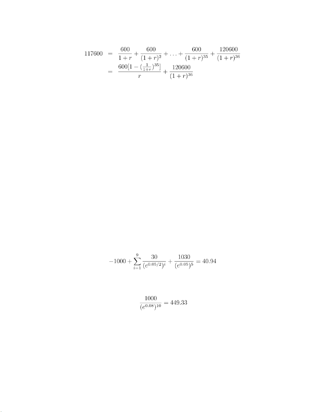
Since the bank charges 2 points, the amount of money we receive for
this loan is actually 120,000 × 0.98 = 117,600. The interest we need to pay per month is 120,000 ×
0.5% = 600. Therefore the cash flow sequence of this loan is 11 time (mths) 0 1 2 ... 35 36 cash flow
117600 -600 -600 ... -600 -120600 lOMoARcPSD|359 747 69
Let r be the effective interest rate per month for this loan, then
We can solve the above to get r ≈ 0.5615%. 4.13
The present value of paying the entire amount of $16,000 now is
simply $16,000, while the present value of paying $10,000 now and another
$10,000 at the end of ten years is
S = 10,000 + 10,000(e−r)10 Therefore
(a) r = 0.02, S = 18,187.31, which is not preferable. (b) r
= 0.05, S = 16,065.31, which is not preferable.
(c) r = 0.10, S = 13,678.79, which is preferable.
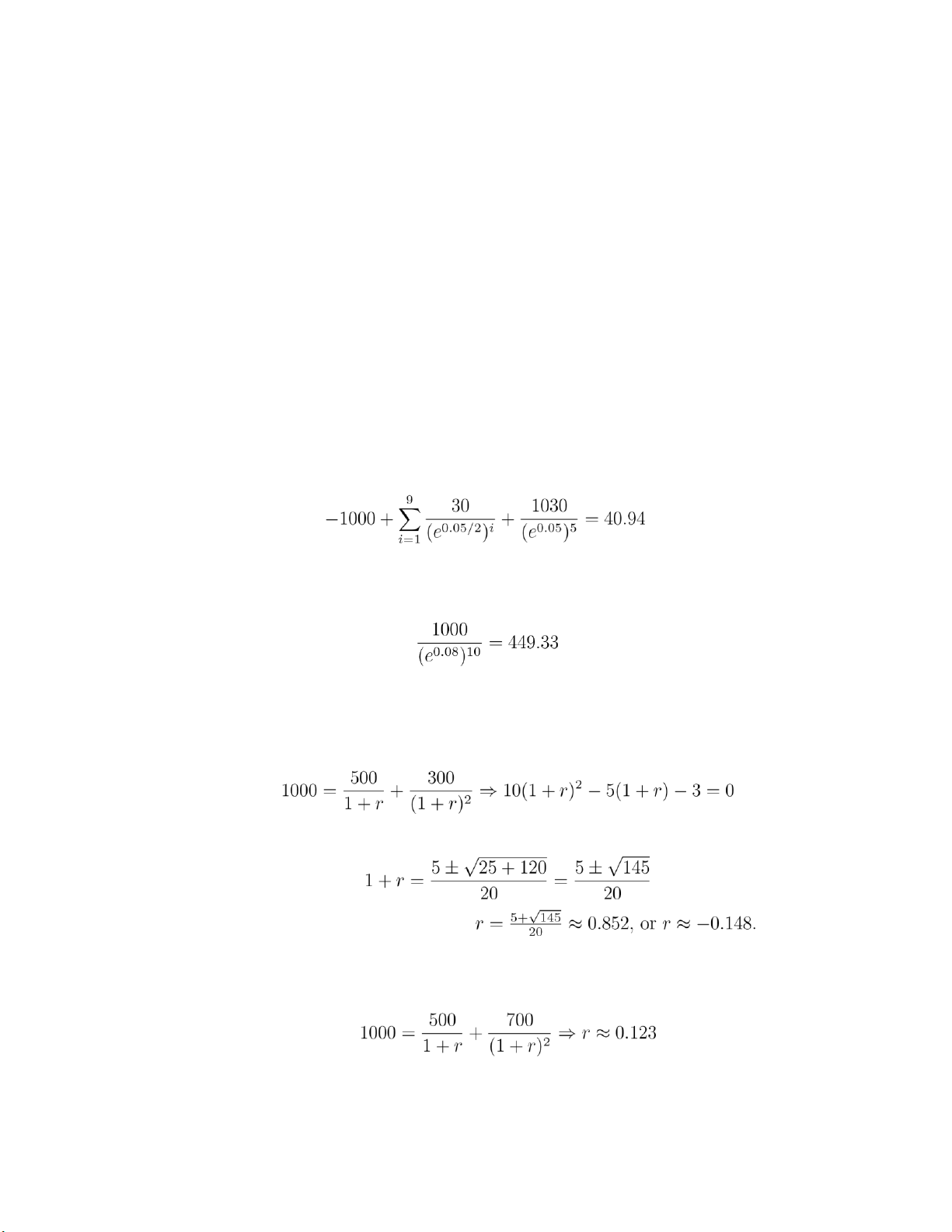
4.14 The cash flow sequence is as follows,
time (yrs) 0 0.5 1 ... 4.5 5 cash flow -1000 30 30 ... 30 1030
With a continuously compounded interest 5%, the present value of above is
4.15 The present value of a cash flow of 1,000 at the end of 10 years with a
continuously compounded interest rate 8% is
4.16 The rate of return is the effective interest rate which makes the present value of
the cash flow streams equal to the initial payment. Therefore lOMoARcPSD|359 747 69
4.15 (1 + 05/n)n would be the amount on deposit after one year if 1 is initially deposited, the
nominal interest rate is 5 percent, and interest is compounded n times in the year. The more times
it is compounded the higher this amount should be.
4.16 The amount of interest earned after n days is 100(e.06n/365 − 1).
4.17 1000e3r + 2000e2r + 3000er
4.18 You would pay the present value of the string of payments: 1. 4.19 When 20 +
. That is, when r > .2. 4.20
104e−r = 110e−2r
giving that er = 110/104 or r = log(110/104) = .0561 4.21
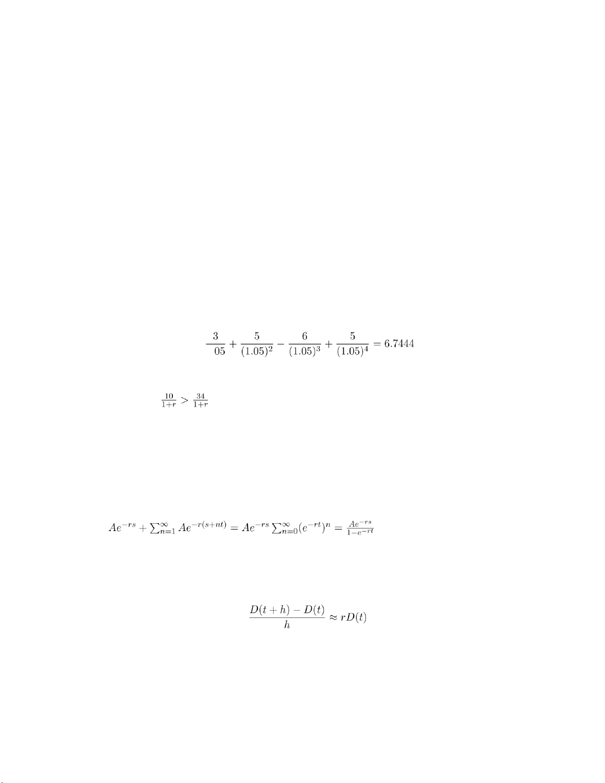
4.22 (a) The interest earned by time t+h on the interest earned in (t,t+h) is of smaller order than h. (b) From (a), we have
Letting h → 0, the approximation becomes exact and we obtain that
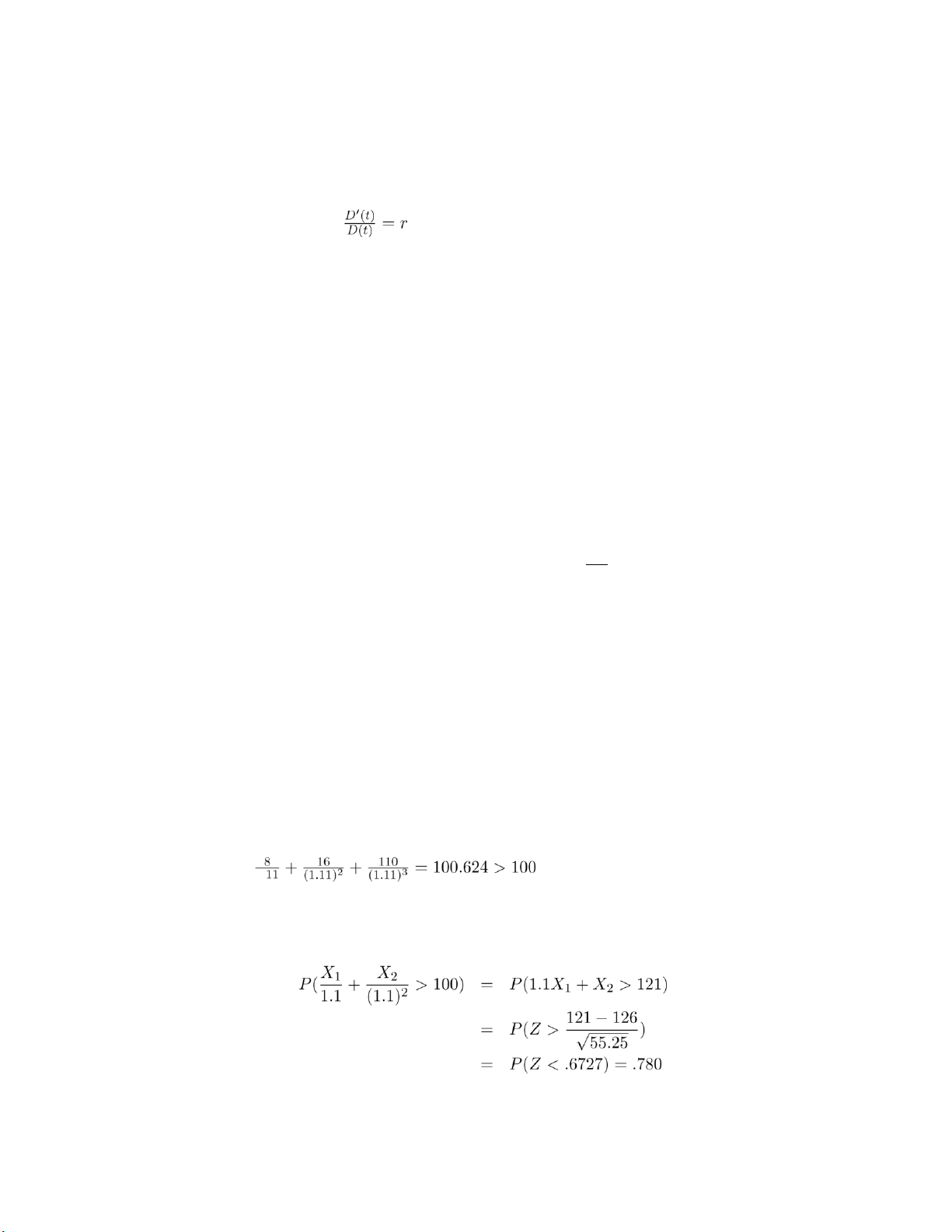
D′(t) = rD(t) 5 lOMoARcPSD|359 747 69 (c) Integrating both sides of , yields that
log(D(t)) = rt + C or
D(t) = Kert
for some constant K. Evaluating at t = 0 gives D = D(0) = K.
4.23 By Proposition 4.2.1, the cash flow 100,140,131 is preferable for any positive interest rate.
4.24 (a) 110/(1 + r)2 = 100 or r = .0488
(b) If R is the rate of return, then R is equally likely to be √1.2−1 or 0. Hence, E[R] = .0477.
4.25 1000e−.8 = 449.33
4.26 100 = 40(1 + r)−1 + 70(1 + r)−2 yielding that r = .0498
4.27 (a) No, it is greater than 10 percent if and only if
i xi/(1.1)i is greater than 1. (b) yes because 1 . . P 4.28 6 lOMoARcPSD|359 747 69
where the preceding used that 1.1X1 + X2 is normal with mean 126 and variance 55.25
5.1 (a) The present value of your net return is 10e−.12 − 10 = −1.1308 (b) −10
5.2 (a) -5;(b)2e−.03 − 5 = −3.059
5.3 Because the call option will be exercised, purchasing it costs C at time 0 and then costs K at
time 1 with the result being owning the security at time 1. Another investment that yields the
security at time 1 is to purchase it at time 0 for its initial price s. By the law of one price
s = C + Ke−r
giving that C = s − Ke−r.
5.4 If C > S an arbitrage is effected by simultaneously selling the call and buying the security.
5.5 Because P ≥ 0, the put call option parity implies that Ke−rt ≥ S − C
5.6 Use Exercise 5.5 to obtain C ≥ S − Ke−rt = 30 − 28e−.05/3
5.7 (a) is not necessarily true (to see this, let K be exceedingly large); (b) is true for if P > K an
arbitrage can be effected by selling the put.
5.8 This follows from the put call option parity formula.
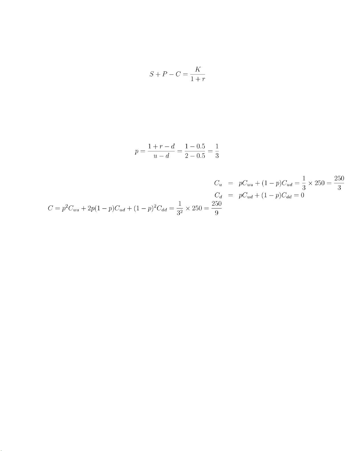
5.10 Buying the security, buying the put, and selling the call has an initial cost of S + P − C and no
matter what the price at time t yields K at that time. (If S(t) ≤ K then the sold call is worthless and 7 lOMoARcPSD|359 747 69
we exercise the put to sell the security for K. If S(t) > K then the bought put is worthless but the
purchaser of the call will exercise and we will receive K for the security.) A second investment that
yields K at time t is to ;put Ke−rt in the bank at time 0. The parity formula now follows from the law of one price.
5.11 (a) K; (b) If P is cost of put then law of one price yields s + P = Ke−rt, giving that P = Ke−rt −s.
(Note that if Ke−rt < s then sert > K > S(t), showing that selling the security with the intention to
purchase it at time t yields an arbitrage.)
5.12 Buying both yields 1 at time t, as would putting e−rt in the bank at time 0. Hence, the law of
one price gives C1 + C2 = e−rt
5.13 Because 25 = S+P −C > Ke−rt = 20e−.1/4, an arbitrage is effected by selling the security, selling
the put, and buying the call. This yields 25 and will cost you 20 at time t.
5.14 If C and P are the costs for the European versions, then Ca = C and Pa ≥ P. The put call parity formula yields
S + Pa − Ca ≥ Ke−rt
5.15 First note that P1 ≥ P2 for if P1 < P2 an arbitrage is effected by buying the P1 put and selling the
P2 put. So assume that P1 ≥ P2. If K1 − K2 < P1 − P2 then an arbitrage is effected by selling the K1,P1
put and buying the K2,P2 put. This has an immediate return of P1 − P2. If the sold put is exercised at
time t then if you also exercise the bought put you will have to pay K1 − K2, which is less than your immediate return. 8 lOMoARcPSD|359 747 69
5.16 If it were less than could buy the exercise time t put and sell the exercise time s < t put. If the
sold put is ever exercised then you should exercise the bought put at that time. These latter
transactions cancel each other and you have the initial difference in prices as your arbitrage.
5.17 (a) True because it is clearly true for an American call option and the European is worth the same amount.
(b) This is only true if the domestic interest rate is at least as large as the foreign rate. (c) This
need not be true since it is sometimes optimal to exercise early and so being forced to continue can be detrimential.
5.18 (a) If the security has a lot of volatility.
5.19 s − d 5.20 .
5.21 If not then an arbitrage would result from buying the one with lower strike and selling the one with higher strike. 5.22 (a) negative
5.23 Suppose you buy the K = 110 call and sell the K = 100 call. This would give you 20 − C at time
0 and would cost at most (if the sold option is exercised then you should exercise the other option)
10 at exercise time t. So there would be an arbitrage if 20 − C ≥ 10e−rt. Hence, C ≥ 20 − 10e−rt.
5.24 Convexity follows from the analogous result for call options upon using the put call option parity formula. 9 lOMoARcPSD|359 747 69
5.25 yes, to show that having λ put options with strike K1 and 1 − λ put options with strike K2 is
better than having one put option with strike K = λK1 +(1−λ)K2 exercise the put pair at the same
time that the single put is exercised, taking (K∗ −s)+ as the return from exercising a K∗ strike put
when the security price is s.
5.26 If s is the price at time t1 than better than exercising is to sell the security at that time and
then exercise and give back the security at time t2. This follows because exercising at time t1 gives
a time t1 return of s−K1, whereas the latter policy gives a time t1 return of s−K2e−r(t2−t1).
5.27 This follows because
S(t) − max(K,S(t) − A) = S(t) + min(−K,−S(t) + A) = min(S(t) − K,A) where we used
that −max(a,b) = min(−a,−b). Hence,
(S(t) − max(K,S(t) − A))+ = max{0,min(S(t) − K,A)} = min{(S(t) − K)+,A)}
5.28 A function is concave if the curve obtained when it is plotted is such that the straight line
connecting any two of its points lies below or on the curve.
5.29 An arbitrage is a sure win, so neither is necessarily true. 10 lOMoARcPSD|359 747 69 17
6.1 We need to see whether we can find a probability vector (p1,p2,p3) for which all
bets are fair. In order to have all bets fair, pi = 1/(1 + oi). Therefore, p1 = 1/2 p2 = 1/3 p3 = 1/6
Since the pi’s sum up to 1, (p1,p2,p3) is indeed a probability vector which makes all bets fair.
Therefore, no arbitrage is present.
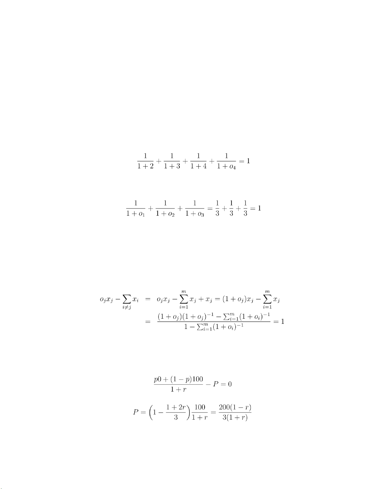
6.2 To rule out the arbitrage opportunity, o4 must satisfy the equation,
Therefore, o4 = 47/13.
6.3 No arbitrage is present since
6.4 If no arbitrage is present, then (p1,p2,p3) = (1/2,1/3,1/6) has to be the probability
vector which makes all bets fair. Therefore
o12(p1 + p2) − p3 = 0 ⇒ o12 = 1/5
o23(p2 + p3) − p1 = 0 ⇒ o23 = 1
o13(p1 + p3) − p2 = 0 ⇒ o 13 = 1/2
6.5 If the outcome is j, then the betting scheme xi,i = 1,...,m, gives me
6.6 From Example 6.1b, p = (1+2r)/3. The payoff of the put option is 0 if the stock price
goes up, and 100 if the stock price goes down. To rule out arbitrage, the expected return
of buying one put option under the probability distribution has to be zero. That is, Therefore 18 The put-call parity says lOMoARcPSD|359 747 69
In this example, one can check the following indeed holds. 6.7
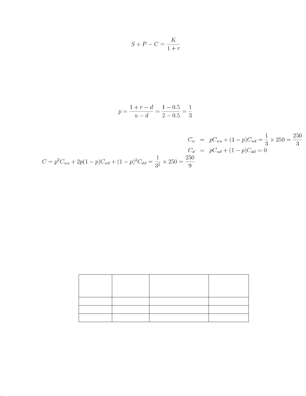
Since the call option expires in period 2 and the strike price K = 150, it is clear that Cuu = 250 Cud = 0 Cdd = 0
Let p denote the risk neutral probability that the price of the security goes up, then
where we assume r = 0. Then we can find C by computing the expected return of the call
option in the risk neutral world.
6.8 See Example 8.1a for details.
6.9 We need to find a betting strategy which gives a weak arbitrage if (a) C = 0 and (b) C = 50/3.
(a) C = 0. In this case it is clear that buying one share of stock is a weak arbitrage. At
time 0, one does not have to pay out anything. At time 1, the profit is 50 if the stock
goes up to 200, and 0 if the stock price is either 100 or 50.
(b) C = 50/3. In this case it is not that clear how a weak arbitrage can be established.
But since the price of the call option is high, it’s intuitive that we want to sell it. So,
let’s consider a portfolio consisting of selling one share of the call option and buying
x share(s) of the stock. Our return depends on the price of stock at time 1, which is tabulated as follows. stock balance value of the portfolio profit price at time 1 at time 0 at time 1 (r = 0) 200 50/3 − 100x −50 + 200x 100x − 100/3 − 100 50/3 − 100x 0 + 100x 50/3 − 50 50/3 100x 0 + 50x 50x + 50/3
From the above table, if we choose x = 1/3, then the profit is 50/3 if the stock price
is 100 at time 1, and 0 otherwise, which is a weak arbitrage.
6.3 (a) There is no arbitrage if there are probabilities p such that 1,p2,p3 Pi pi = 1 and lOMoARcPSD|359 747 69
4p1 + 8p2 − 10p3 = 0 and
6p1 + 12p2 − 16p3 = 0
Because the first equation implies that 6p1 + 12p2 − 15p3 = 0, any solution must have p3 = 0.
Consequently, p1,p2 would need to satisfy p1 +2p2 = 0 which is impossible because the pi must be
nonnegative. Hence, an arbitrage is possible. One such is to let x1 = 1.5,x2 = −1. (b) No arbitrage if
there are probabilities p1,p2,p3 such that Pi pi = 1 and 6p1 − 3p2 = 0
−2p1 + 6p3 = 0
10p1 + 10p2 + xp3 = 0
Hence, p2 = 2p1, and p1 = 3p3 Using that i pi = 1, this yields that p1 = .3, p2 = .6, p3 = .1. Therefore, no
arbitrage is possible if x = −P90.
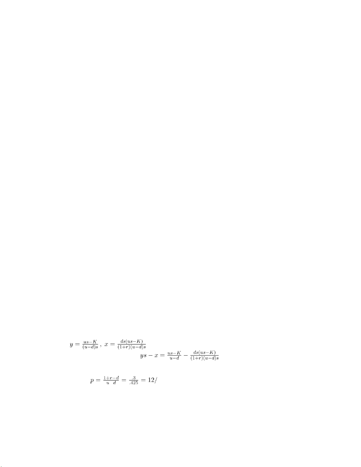
6.10 Let S(0) = s and suppose that us > K > ds. If you purchase y shares of the security by borrowing
x and investing the remaining ys − x then your payoff at time t is payoff = ( −− yus (1 + r)x, if S(1) = us yds (1 + r)x,
if S(1) = ds
Hence, the payoff from the option is replicated if we choose x,y so that
yus − (1 + r)x = us − K
and yds − (1 + r)x = 0 Setting
does the trick. It now follows, by the law of one price, that the
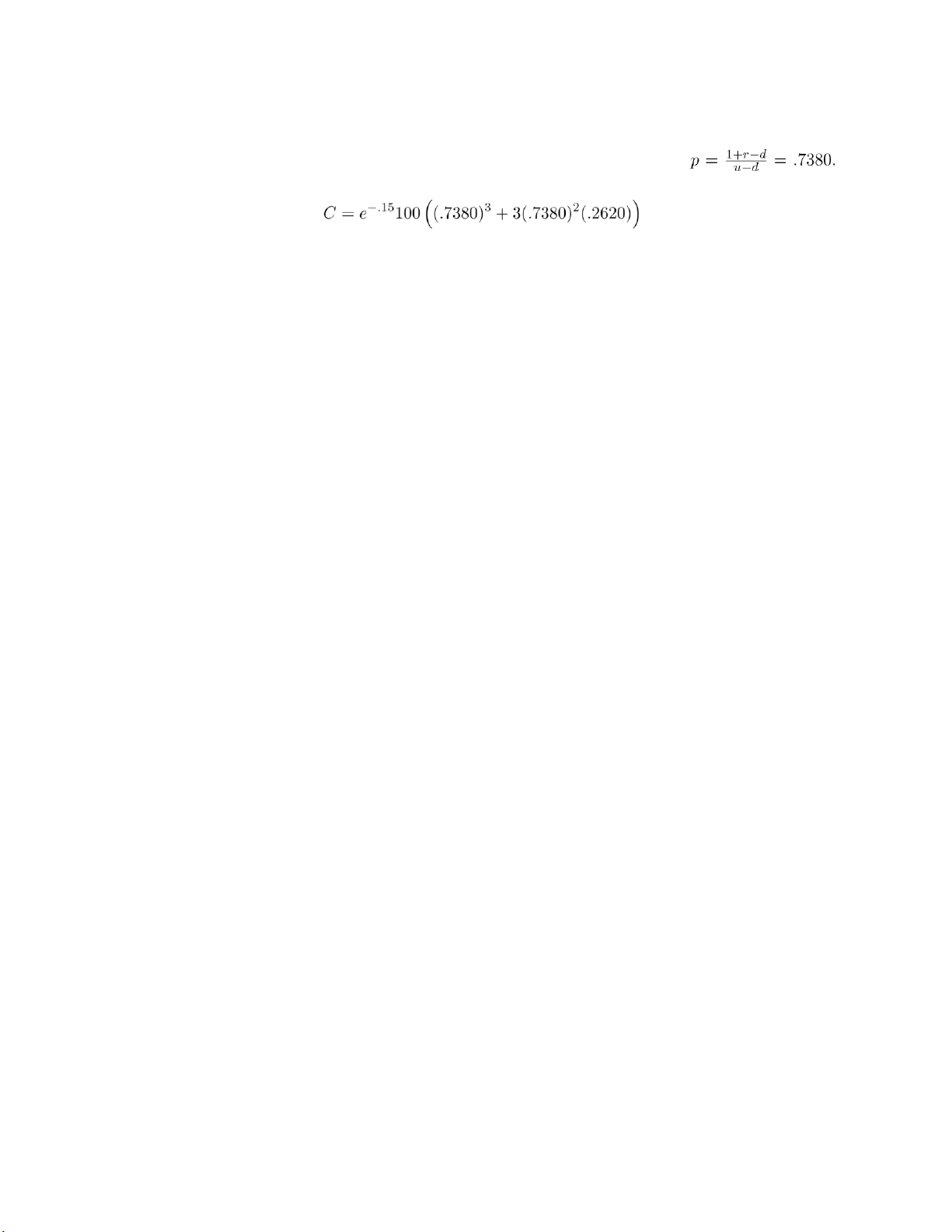
no arbitrage cost of the option is . 6.11 (a) With
17, the expected payoff is 25(1 − p)2p3 = .7606 , so the no
arbitrage cost is .7606(1− .1)−5 = .4723 (b) yes
(c) 25(1/2)5 = 25/32 = .78125 lOMoARcPSD|359 747 69 11
6.12 No arbitrage is possible if new bet is fair when the up probability is
The bet will pay off if at least 2 of the first 3 moves are up moves. Hence, no arbitrage if 12 19 lOMoARcPSD|359 747 69 7.1 7.2
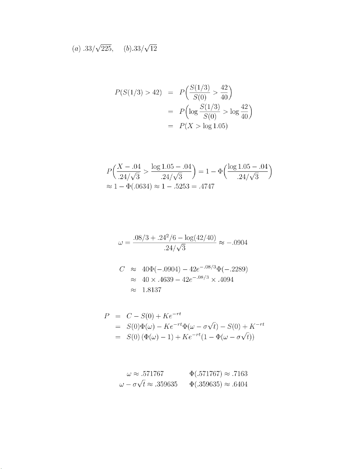
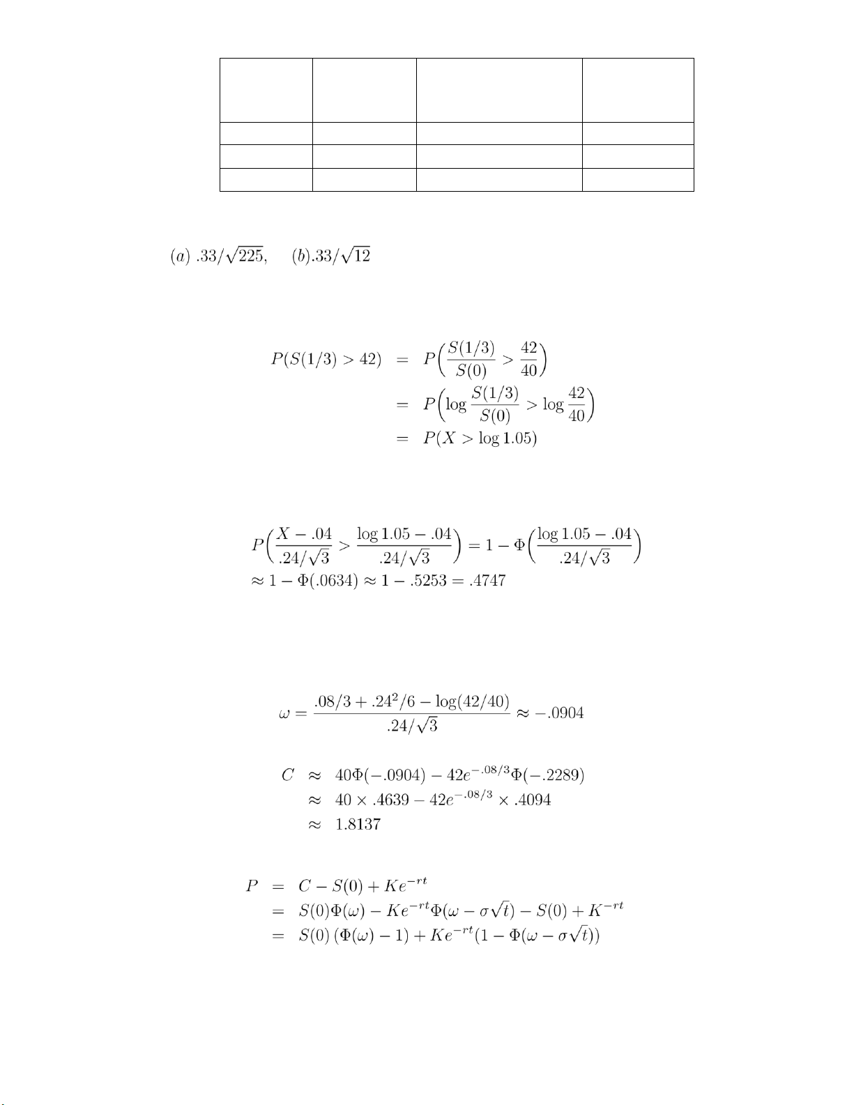
Since the unit of time is one year, t = 4/12 = 1/3. The probability that the
call option will be exercised at t = 1/3 is the probability that the stock price at t = 1/3 is
greater than the strike price K = 42, which is
where X is a normal random variable with mean µt = .12/3 = .04 and standard deviation
σ√t = .24/√3. Therefore, the above probability is equal to 7.3 The parameters are t = 1/3 r = .08 σ = .24 K = 42 S = 40 so we have that Therefore,
7.4 From the put-call parity, we can derive the no-arbitrage cost to a put option
where ω is defined in equation (7.7) in text (page 87). The parameters are K = 100 S(0) = 105 r = .1 σ = .30 t = 1/2 lOMoARcPSD|359 747 69
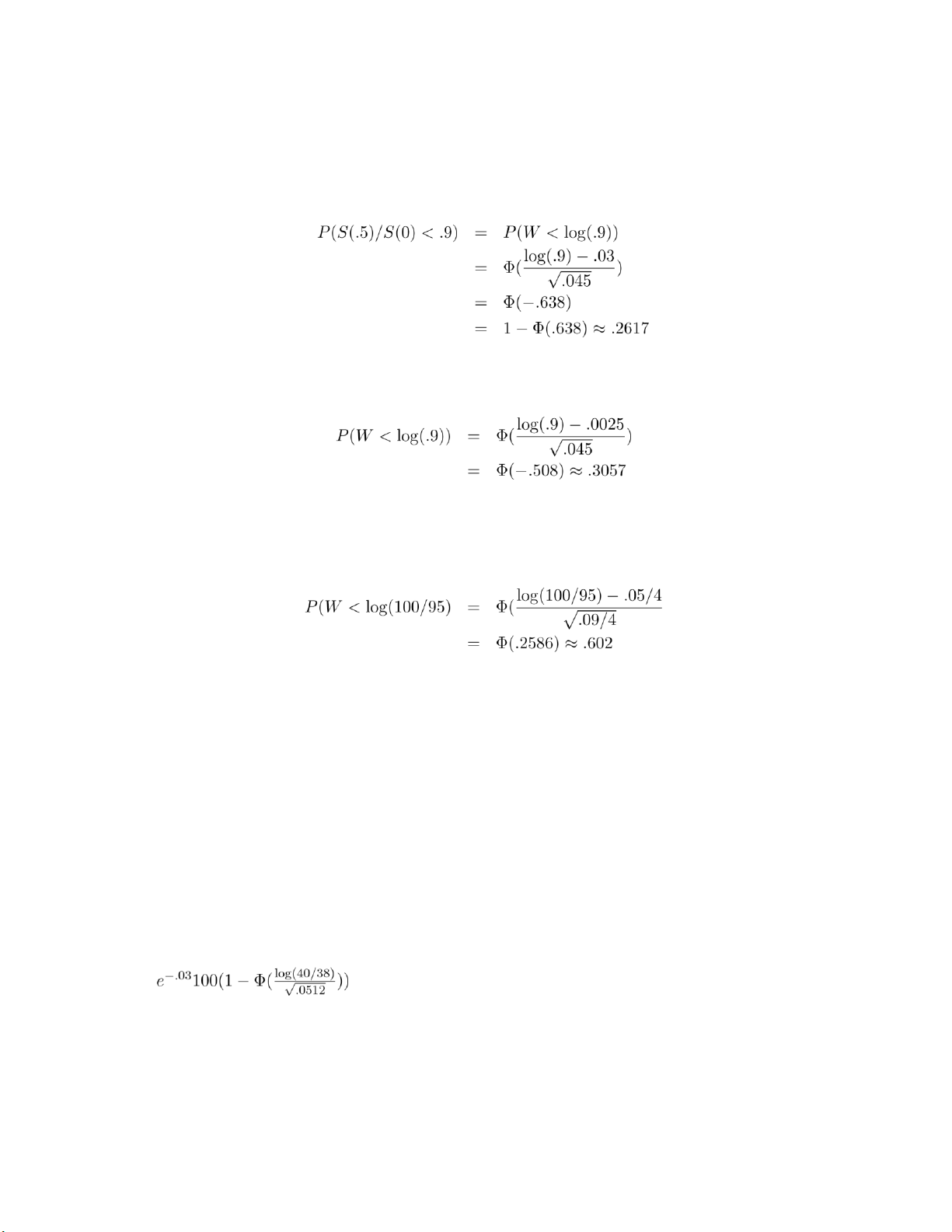
7.5 (a) With W being a normal random variable with mean .03 and variance .045
(b) Now we use the risk neutral drift r − σ2/2 = .05 − .045 = .005. With W being a normal random
variable with mean .0025 and variance .045
7.6 (a) Use formula in text.
(b) With W being a normal random variable with mean .05/4 and variance .09/4
(c) The risk neutral drift is r − σ2/2 = −.005. With W being a normal random variable with mean
−.0025 and variance .045 the no arbitrage cost is 50e−.04P(W > log(105/95))P(W > 0).
7.7 With W being a normal random variable with mean (.06−(.32)2/2)/2 = .0044 and variance
(.32)2/2 = .0512 the risk neutral valuation is
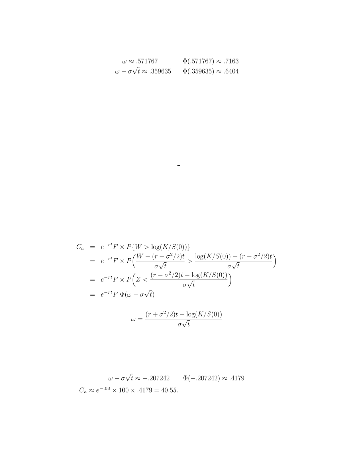
e−.03100P(W > log(40/38)) = e−.03100(1 − Φ(.207)) ≈ 40.55 7.8
7.9 No, you also need to know the drift of the geometric Brownian motion. 13 lOMoARcPSD|359 747 69
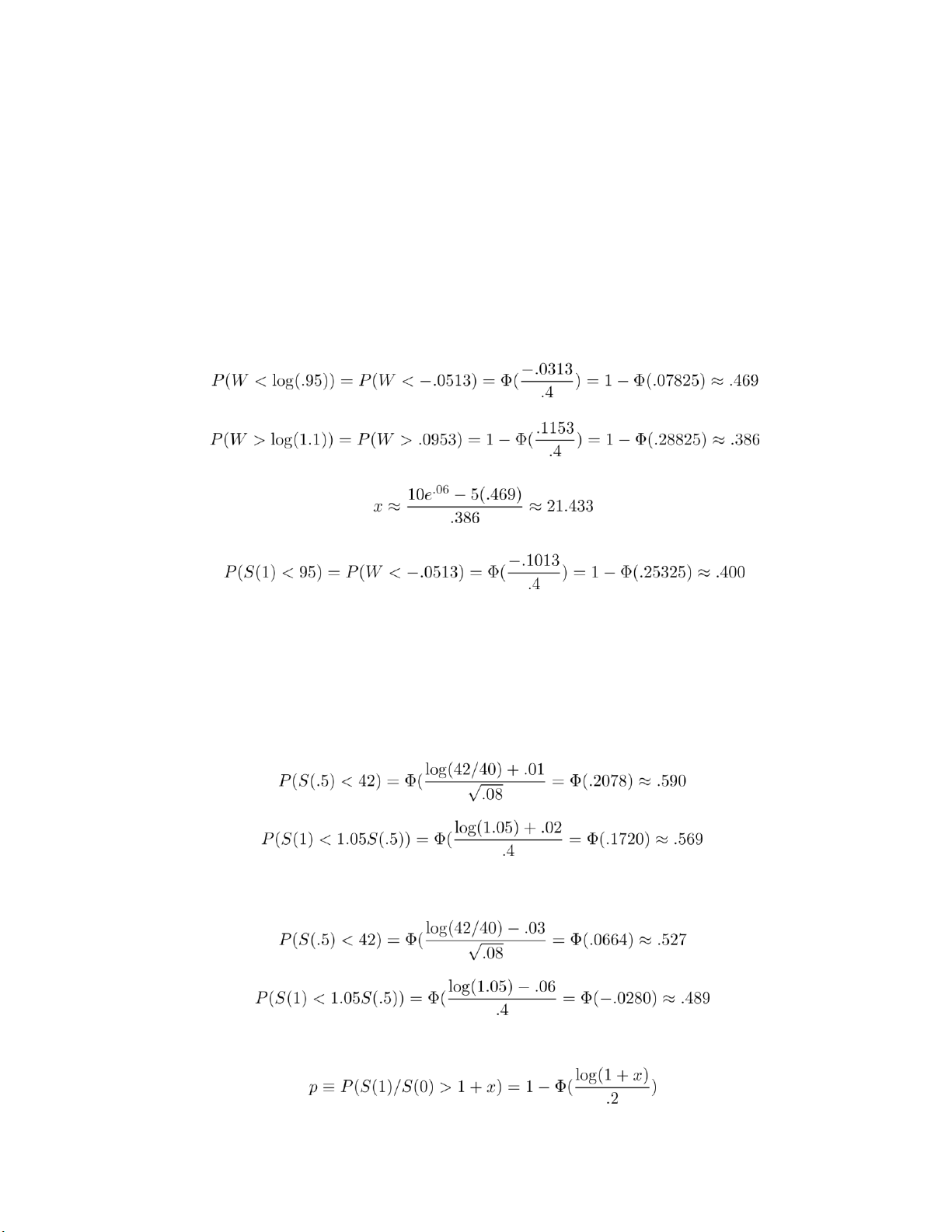
7.10 (a) The risk neutral geometric Brownian motion has drift r − σ2/2 = .06 − .08 = −.02.
No arbitrage if under the risk neutral geometric Brownian motion. Under this process
W ≡ log(S(1)/S(0)) is normal with mean −.02 and variance .16. Hence, no arbitrage if
10 = e−.06 (5P(W < log(.95)) + xP(W > log(1.1))) Now, and Hence,
(b) Using that the actual mean of W is .05 yields that
7.11 (a) The risk neutral drift is −.02. There is no payoff with probability given by
P(S(.5) < 42,S(1) < 1.05S(.5)) = P(S(.5) < 42)P(S(1) < 1.05S(.5)) Under the risk neutral GBM,
Hence, there is no payoff with probability approximately .336, yielding that the expected payoff at
time 1 is 66.4. Hence, there is no arbitrage if C ≈ e−.0666.4 ≈ 62.53. (b) Using the actual drift
Hence, the investment will make money with probability 1 − .258 = .742.
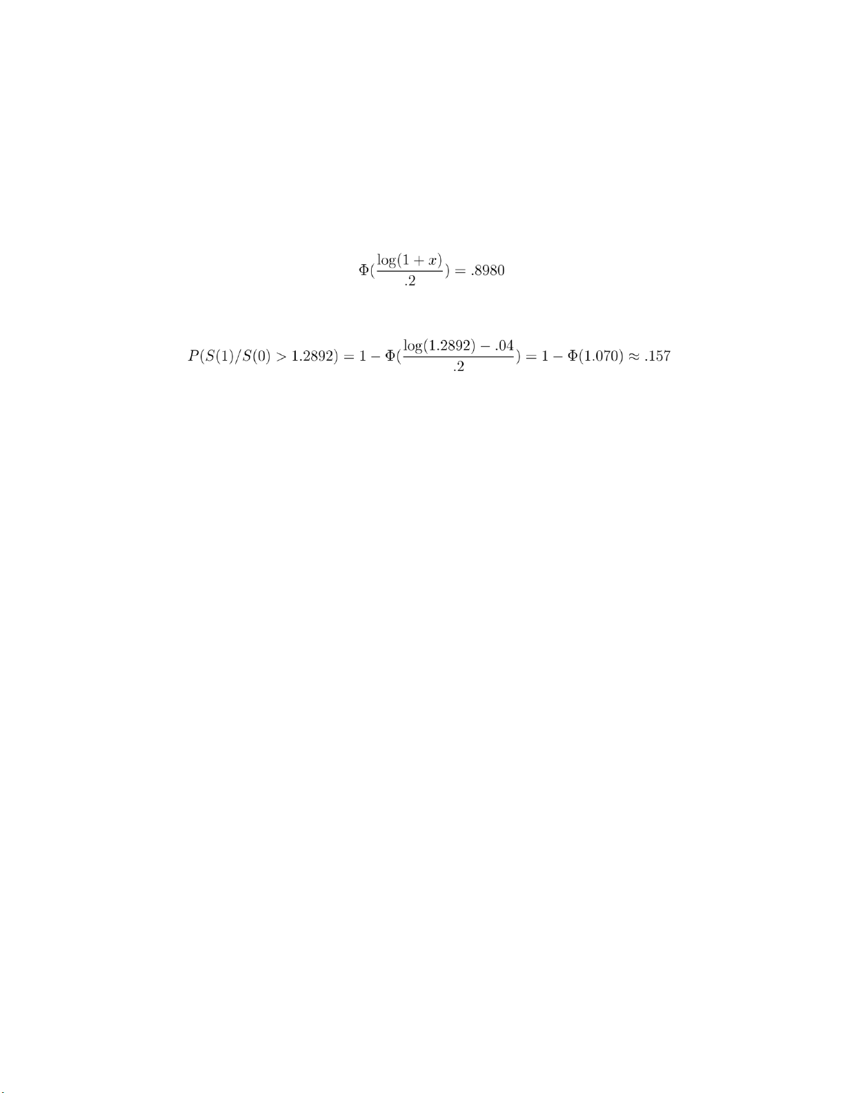
7.12 (a) The risk neutral drift is 0. Under the risk neutral GBM 14 lOMoARcPSD|359 747 69 There is no arbitrage if
10 = e−.02100p
Thus, there is no arbitrage if p = .1020, yielding that
Using that Φ(1.27) = .8980 yields that log(1 + x) = .254 or x = .2892. (b) Using the actual drift
7.13 Lemma 7.5.3 gives the result. 7.14 S(0) 7.15 S(0)
7.16 The price at time t converges to S(0)ert as the volatility goes to 0. So the cost should be
e−rt(S(0)ert − K)+ = (S(0) − Ke−rt)+.
7.18 Not necessarily concave nor convex. 8.1 yes
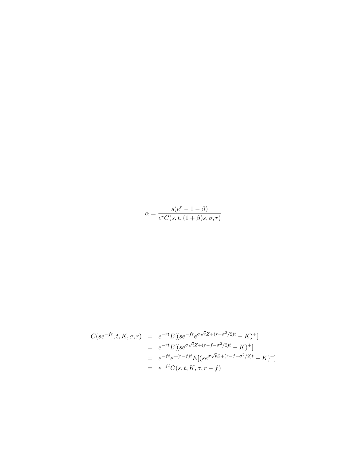
8.2 Geometric Brownian motion with drift r − σ2/2 − f and volatility σ.
8.3 C(s(1 − f)2,K,t,r,σ) 15 lOMoARcPSD|359 747 69
8.4 Because one should never exercise a call option early when there are no dividends it follows
that one should never exercise earlier than td or after td but before t.
8.5 The payoff form the capped option is the difference between the payoff from at K,t call and the
payoff from a K + B,t call. Hence, by the law of one-price its no-arbitrage cost is C(s,K,t,r,σ) − C(s,K
+ B,t,r,σ).
8.6 Under the risk neutral Geometric Brownian motion, the expected return from this investment is
E[(1 + β)s + α(S(1) − (1 + β)s)+] = (1 + β)s + αerC(s,t,(1 + β)s,σ,r)
This bet won’t give rise to an arbitrage provided the preceding is equal to ser. Thus,
8.7 Under the risk neutral Geometric Brownian motion, provided that K > (1 + β)s, the expected
return from this investment is
E[(1+β)s+(S(1)−(1+β)s)+−(S(1)−K)+] = (1+β)s+erC(s,t,(1+β)s,σ,r)−erC(s,t,K,σ,r)
There is no arbitrage provided the preceding is equal to ser, which will be the case under the stated
condition. Because s(1 + β)e−r − s < 0, and C(s,t,K,σ,r) is decreasing in K, the condition that K will
exceed s(1 + β) is satisfied.
8.8 With Z being a standard normal random variable
8.9 (a) Rather than exercising at time s < t1, and thus paying K1 at time s, a dominating strategy is to
exercise at time t1 and thus pay K1 at time t1.
(b) This follows because C(x,t − t1,K,σ,r) is the value of the call at time t1 when S(t1) = x. 16 lOMoARcPSD|359 747 69
(c) This follows because C(y,t − t1,K,σ,r) is a strictly increasing function of y.
(d) This follows because the optimal policy is to exercise the option to purchase the call optionat
time t1 if and only if S(t1) ≥ x.
8.10 (a) Better than exercising at time t1 is to exercise (no matter what the price) at time t2, since
the only difference is that in the former case you pay the present value amount K1e−rt1 whereas in
the latter case you pay the present value amount K2e−rt2. Hence, if K2e−rt2 < K1e−rt1 you should never
exercise at time t1.
(b) The time t1 risk neutral expected return if the option is not exercised at that time is C(y,t2 −
t1,K2,σ,r) if S(t1) = y. The time t1 value of the option if it is exercised at time t1 is y − K1. Hence, if S(t1)
= y, one should exercise at time t1 if
y − K1 > C(y,t2 − t1,K2,σ,r)
8.12 (a) yes; (b) no; (c) no; (d) yes.
8.15 This option should be exercised whenever the price is at least K. It can be explicitly priced by
using the formula derived in Chapter 3 for the maximum by time t of a Brownian motion. It can be
approximated by a N period binomial model. Take the same states as used in pricing an American
put option, and work backwards to obtain V0(0). It takes a bit less work than determining the risk
neutral cost of an American put option because the optimal strategy for the asset-or-nothing is known in advance.
9.1 With Xi equal to fortune after investment i, we have Investment 2 is better.
9.2 E[X] < 0 so optimal is a = 0. 17 lOMoARcPSD|359 747 69
9.3 The rate of return R is such that
. Hence, R = X1/n −1. Because g(x) = x1/n is concave in
x it follows from Jensen’s inequality that
E[R] = E[X1/n] − 1 ≤ µ1/n − 1
and the result follows because µ1/n − 1 is the rate of return of an investment of 1 that yields µ after n periods.
9.4 The second derivative with respect to α of expected utility is negative, showing the expected
utility as a function of α is concave. As, allowing α to range from −∞ to ∞, its minimum is, when p
< 1/1, obtained when α < 0, it follows by concavity that its value when α = 0 is greater than its
value for α > 0.
9.5 y should be chosen to maximize −.03y − .0025(.04y2 + .0625(100 − y)2). 9.7 E[log(
i αiwXi)] = log(w) + E[log(
i αiXi)] and so the optimal fractions do not depend on w. P P
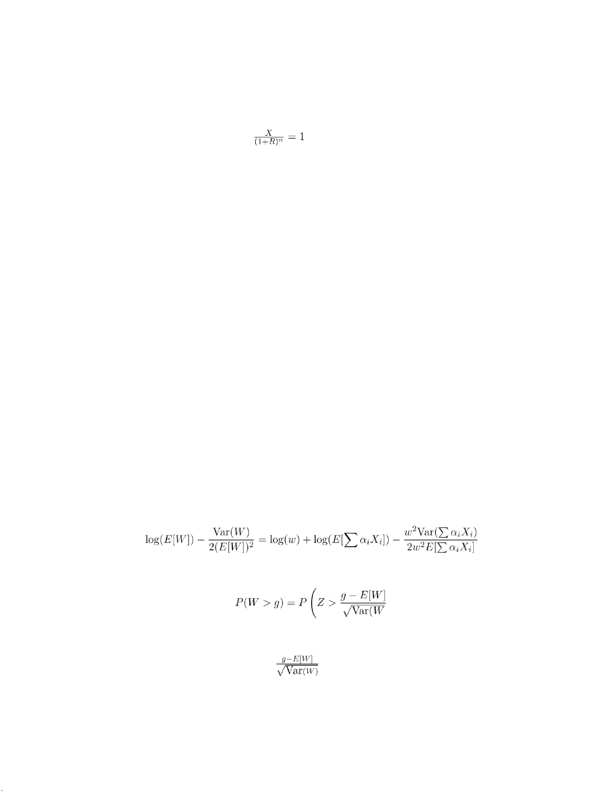
9.9 With W = PwαiXi, we want to maximize Thus, w does not play a role in
determining the optimal αi,i = 1,. .,n.
9.11 With Z being a standard normal !
Hence, want to choose so as to minimize . 18 lOMoARcPSD|359 747 69
9.14 .066 and .076 9.15 Pi αiβi
9.16 ai = (1 − βi)rf, bi = βi, F = Rm.
9.17 (a) Yes, because E[X1 + X2] = 2, we can conclude from Jensen’s inequality that a fixed return of 2 is preferable.
(b) X1 +X2 is preferable to 2X1 because they are both normal and X1 +X2 has the same mean but a
smaller variance than does 2X1.
(c) No, it depends on the utility function. 3X1 has a larger mean but also a larger variance.
(d) Using that −(X1 + X2) is normal with mean −2 and variance 2
E[1 − e−X1+X2] = 1 − e−2+1 = 1 − e−1
whereas, because −3X1 has mean −3 and variance 9
E[1 − e−3X1] = 1 − e−3+4.5 = 1 − e1.5 19 lOMoARcPSD|359 747 69
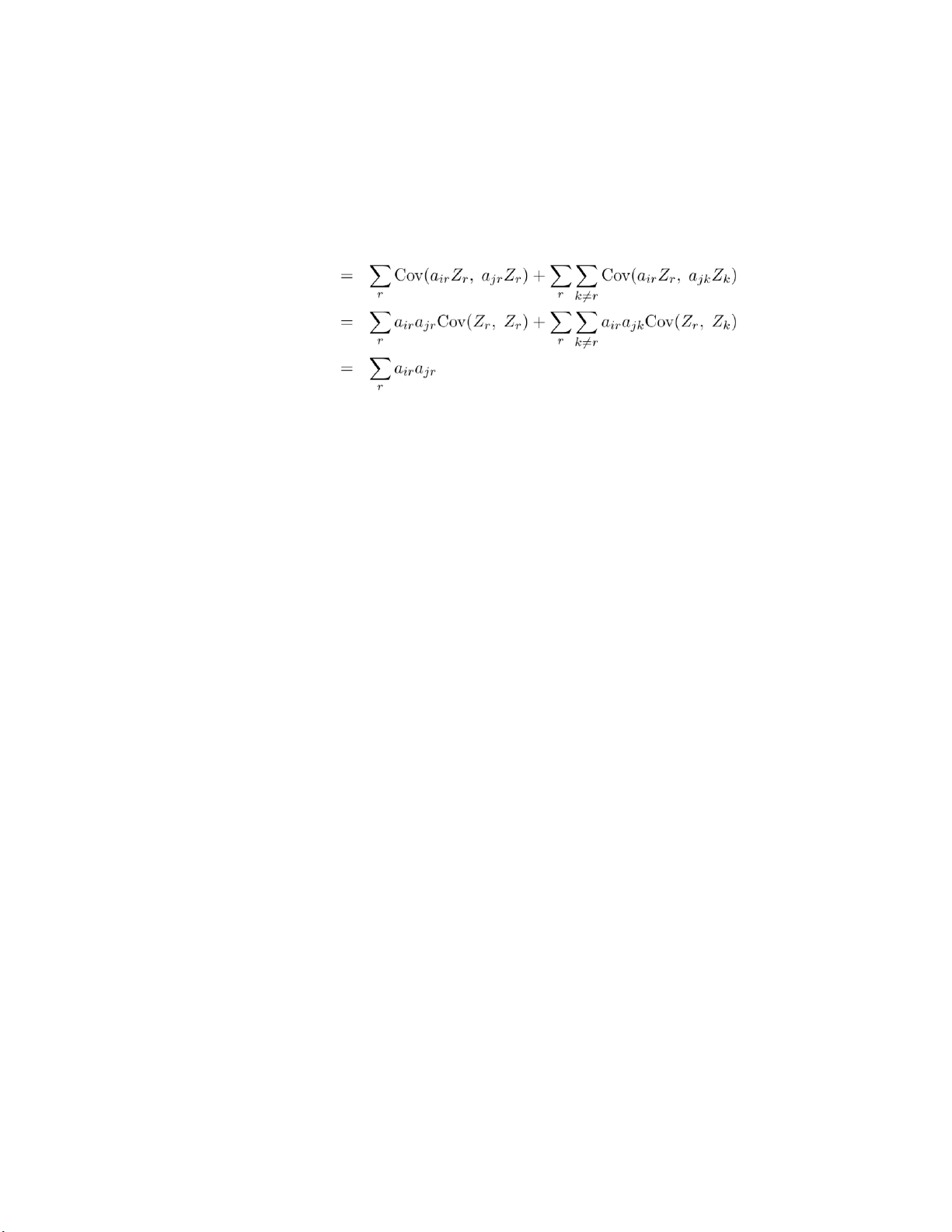
Thus, X1 + X2 is preferable. 9.18 m m Cov(Xi,Xj)
= Cov(XairZr, X ajkZk) r=1 k=1 = Cov(airZr, ajkZk) Xr Xk
where the final equality used that Cov(Zr, Zk) is 1 when k = r and is 0 when k =6 r. 20 lOMoARcPSD|359 747 69
10.1 Immediate by definition.
10.2 Let Ij,j ≥ 1, be independent random variables, each equal either to 1 with probability
p or to 0 with probability 1 − p. Then, n+1 n X Ij ≥ XIj j=1 j=1 which proves the result since
has a binomial distribution with parameters k,p.
10.3 Let Ij,j ≥ 1, be independent random variables, each equal either to 1 with probability p1 or to
0 with probability 1 − p1; and let Jj,j ≥ 1, be independent random variables, each equal either to 1
with probability or to 0 with probability 1
. Assume that the two sequences are
independent of each other. Then,
which proves the result because
has a binomial distribution with parameters n,p2 (true
since IjJj is either 1 with probability p2 or 0 with probability 1 − p2) and has a binomial
distribution with parameters n,p1. 10.4
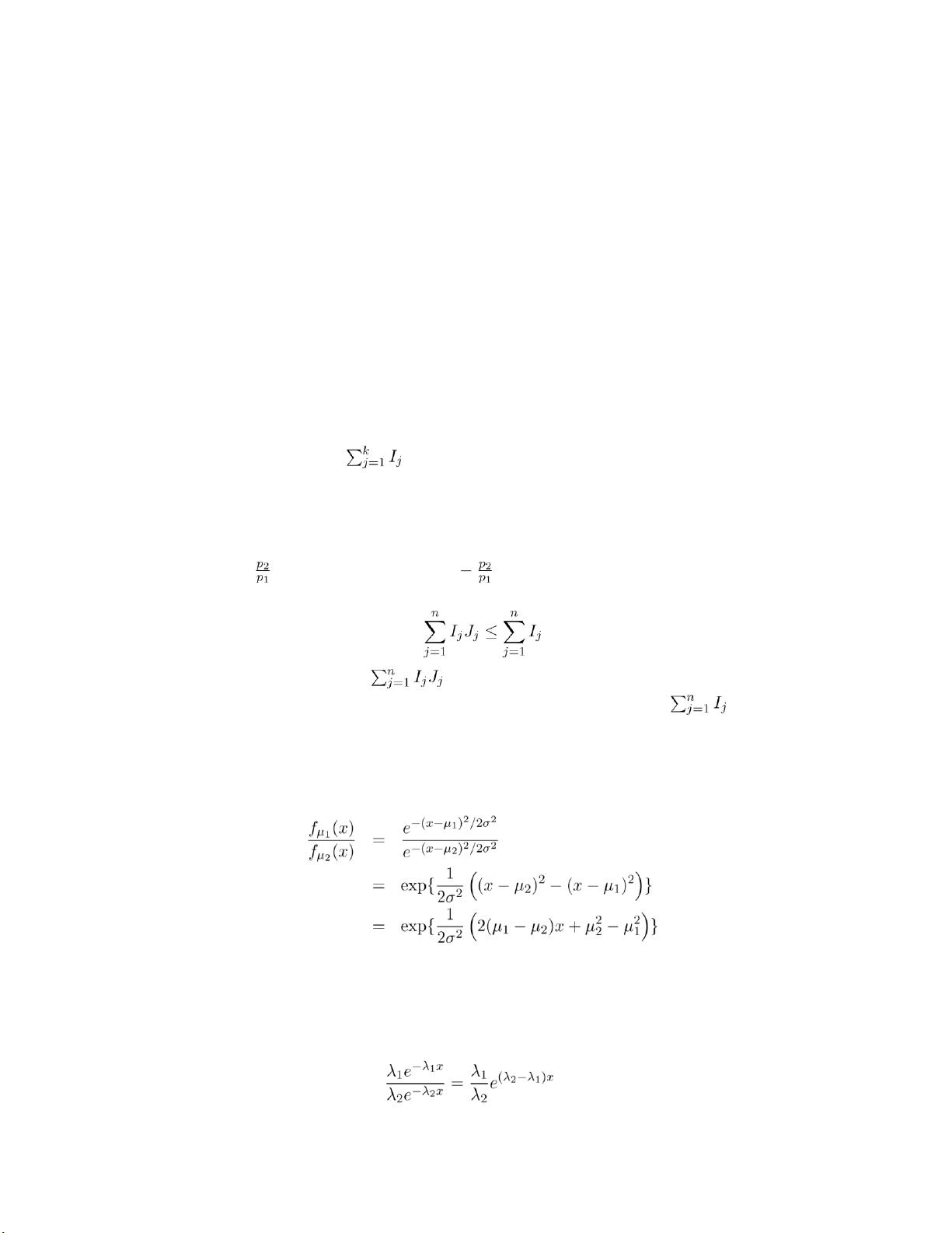
and the preceding is increasing in x when µ1 ≥ µ2. 10.5 21 lOMoARcPSD|359 747 69
and the preceding is increasing in x when λ1 ≤ λ2. 10.6
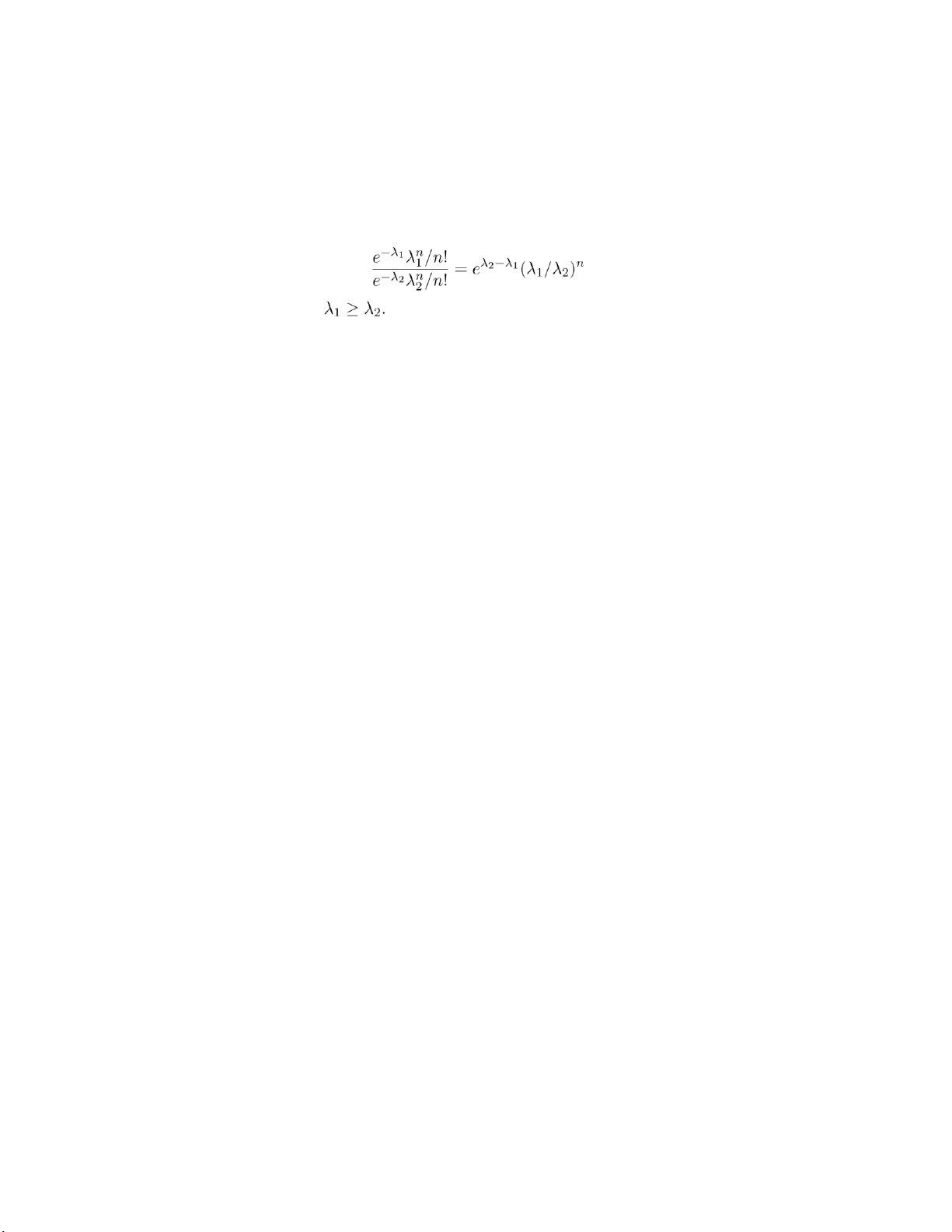
which increases in n when
10.7 This is just Jensen’s inequality.
10.8 Immediately follows from the hint.
10.9 Let h and g both be increasing and concave. We need to show that f(x) ≡ h(g(x)) is
also increasing and concave in x. But
f′(x) = h′(g(x))g′(x)
which is nonnegative since h′ and g′ are both nonnegative because h and g are increasing. Also,
f′′(x) = h′′(g(x))(g′(x))2 + h′(g(x))g′′(x) ≤ 0
where the inequality follows because both terms are nonpositive because h′′ ≤ 0 and h′ ≥ 0 and g′′ ≤ 0.
11.1 Optimal is to invest 2 in project 1 and 4 in project 2. The optimal return is 2log(3) + 2.
11.4 Suppose under the optimal policy that k is invested in project i and r is invested in
project j, where r and k are both positive. Now,
fi(k) − fi(k − 1) ≥ fj(r + 1) − fj(r)
for otherwise investing k − 1 in i and r + 1 in j would, although investing the same amount, yield a
higher return from these two investments. But, by convexity, fi(k + 1) − fi(k) ≥ fi(k) − fi(k − 1) and
fj(r + 1) − fj(r) ≥ fj(r) − fj(r − 1) 22 lOMoARcPSD|359 747 69
showing that investing k + 1 in project i and r − 1 in project j is at least as good as investing k and
r. Continuing in this manner shows that investing k + r in project i and 0 in project j s at least as
good as investing k and r. Continuing with other projects shows that there is an optimal policy that
invests all in a single project.
11.5 (a) Consider a solution that has one value of x equal to k + i and another equal to k
− j where i and j are both positive. (Unless all x equal k this will be the case.) We now argue
that a better solution is given by leaving all other values unchanged and changing k + i to k
+ i − 1 and changing k − j to k − j + 1. That is, we claim that
f(k + i) + f(k − j) ≤ f(k + i − 1) + f(k − j + 1) which is equivalent to
f(k + i) − f(k + i − 1) ≤ f(k − j + 1) − f(k − j)
which follows because f is concave (and k−j+1 < k+i). Hence, we always get a better solution by
letting the x′s become nearer, and in the limit we get that the maximal occurs when all of them are equal.
(b) When f is convex an analogous argument to the one of part (a) will yield the result. This is also
a special case of Exercise 11.4. 11.7 (a) √x
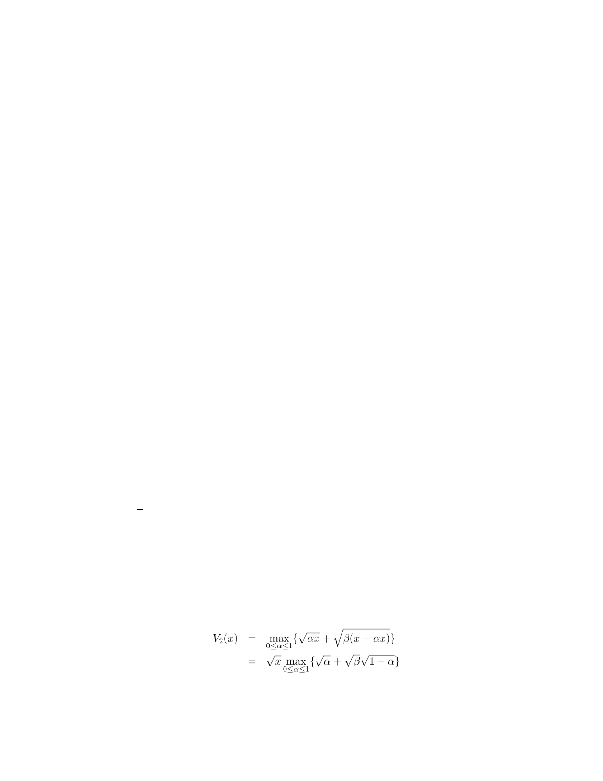
(b) With β = 1 + r, V2(x) = max{√y + V1(β(x − y))} = y≤x (c)
Vn(x) = max{√y + Vn−1(β(x − y))} y≤x
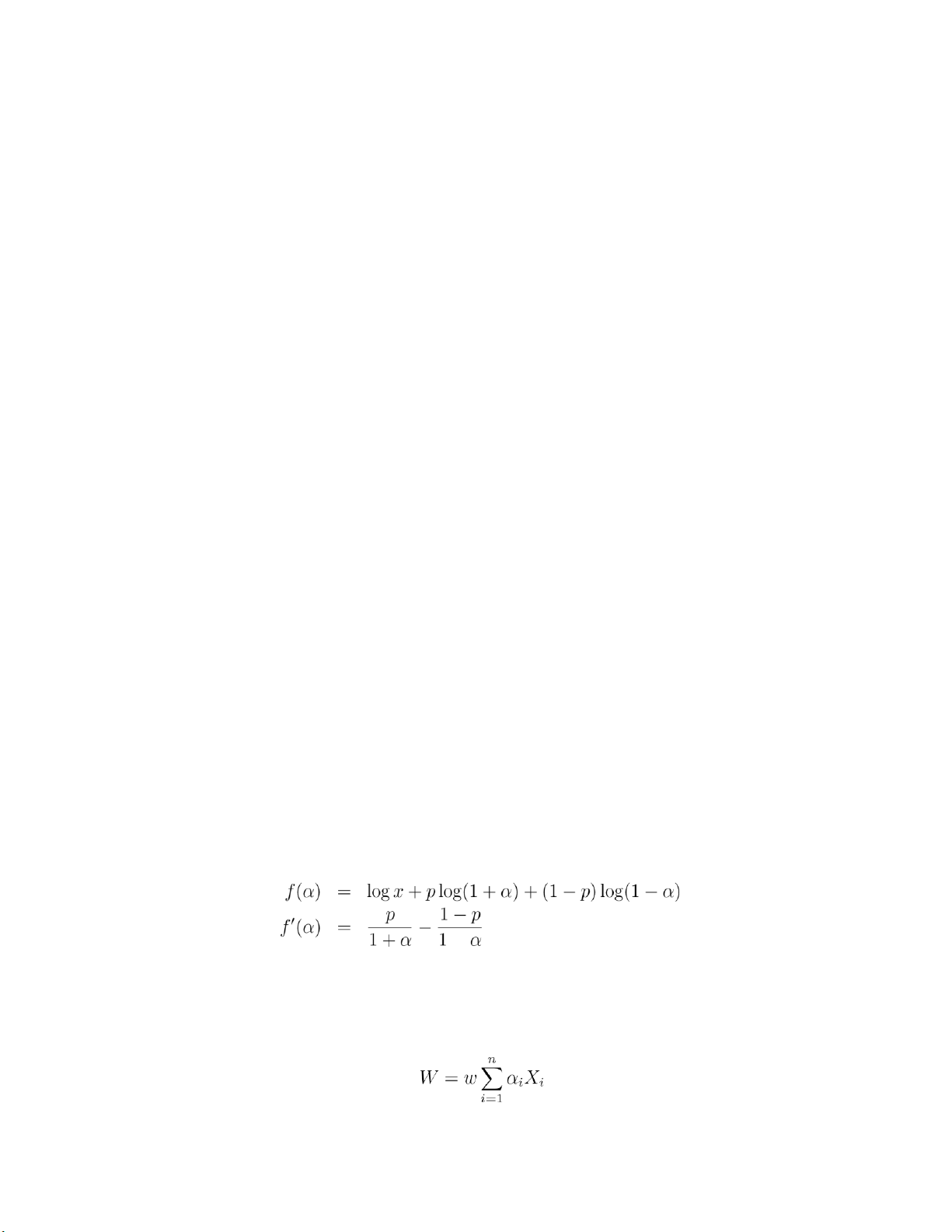
(d) Rewriting so that the decision is the fraction of your wealth that you consume
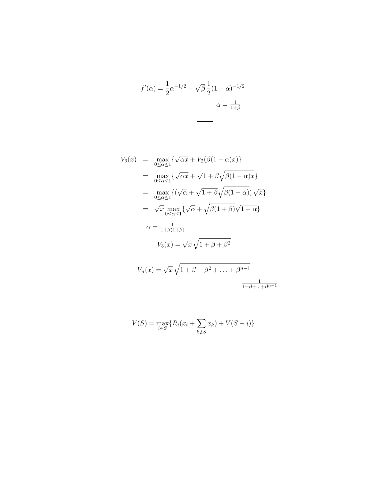
Calling the term inside the maximum f(α) and differentiating yields 23 lOMoARcPSD|359 747 69
Setting equal to 0 yields that the maximum occurs when
, with the optimal value being
V2(x) = p1 + β √x Now,
The value of α that maximizes is , and In general,
and the optimal fraction to consume witn n periods remaining is 11.8 (a)
(b) First solve when S is a one-point set; then when it is a two-point set, and so on.
11.9 In the first investment she should risk .2x if her fortune is x. Her expected utility is log(x)
+ .6log(1.2) + .4log(.8) = log(x) + .0201. In the second investment, she will risk 0 if the win
probability is .4 and .6x if the win probability is .8. Hence, the expected utility of her final fortune
for this investment is log(x) + .3(.8log(1.6) + .2log(.4)) = log(x) + .0578. Hence, the second investment is preferable. 24 lOMoARcPSD|359 747 69
11.11 To determine the minimal time that node j can be reached, let the decision be the node
visited immediately before entering node j. If that node is node i, then if node i is reached at time s
then the time at which node j is reached is s + ts(i,j). Because s + ts(i,j) is increasing in s we would
want to reach node i in minimal time, which proves the equation. 25 lOMoARcPSD|359 747 69
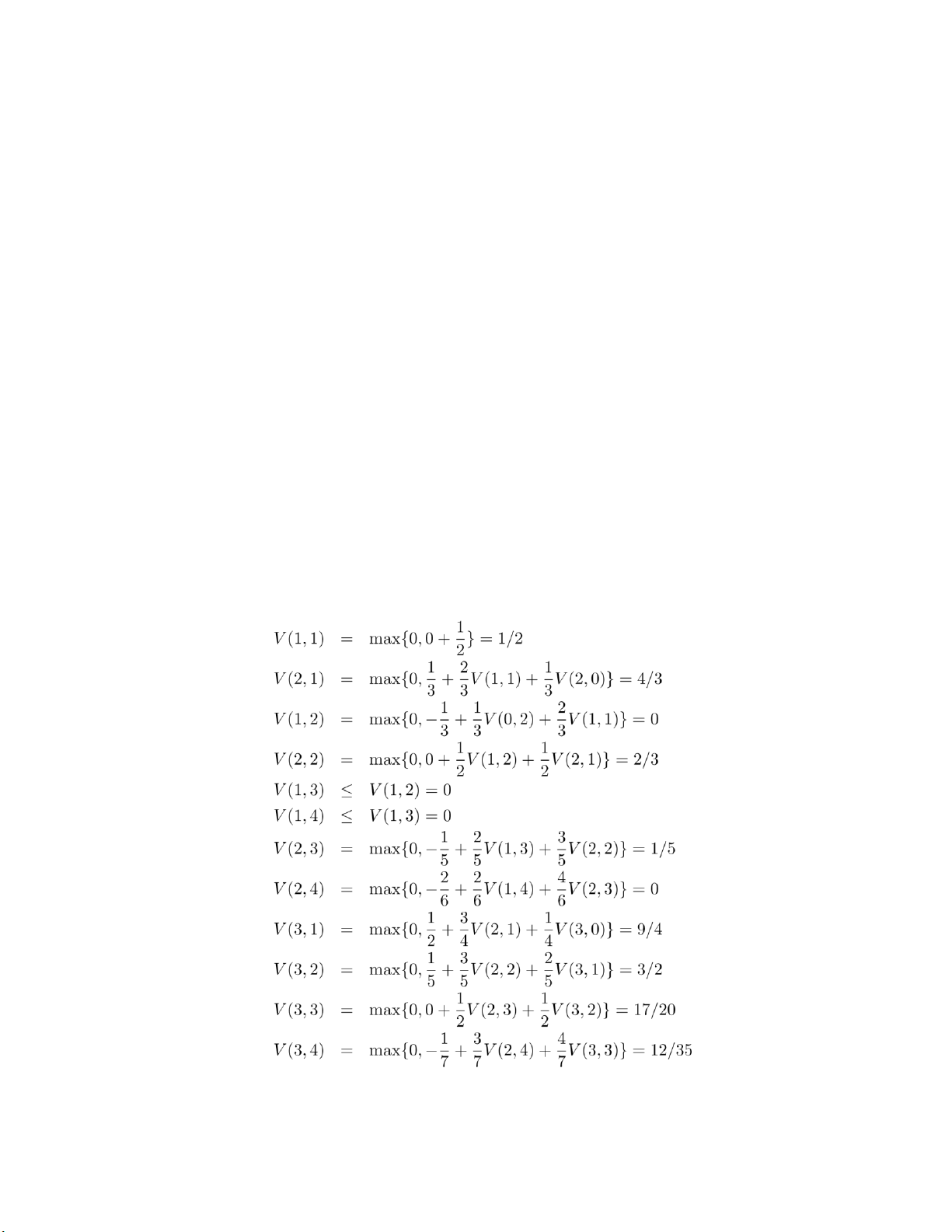
12.1 Letting q(j) = 1 − p(j), then with Vk(n) = 0 if k > n
Vk(n) 1max≤j≤n{p(j)Vk−1(n − j) + q(j)Vk(n − j)} Therefore,
V1(1) = p(1) = .2, a1(1) = 1 V1(2) =
max{p(1) + q(1)V1(1), p(2)} = .4, a1(2) = 2
V1(3) = max{p(1) + q(1)V1(2), p(2) + q(2)V1(1), p(3)} = .6, a1(3) = 3 V2(2) = p(1)2
= .04, a2(2) = 1 V2(3) =
max{p(1)V1(2) + q(1)V2(2), p(2)V1(1)} = .112, a2(3) = 1 V2(4) =
max{p(1)V1(3) + q(1)V2(3), p(2)V1(2) + q(2)V2(2), p(3)V1(1)} = .2096, a2(4) = 1
The maximal probability is .2096. It is optimal to initially invest 1 and then to invest aj(i) when you
are in position where you still need j machines and you have i remaining units to spend.
12.2 With V (i,0) = i, V (0,i) = 0, 26 lOMoARcPSD|359 747 69
12.3 Use mathematical induction to complete the proof. When E[Y ] < 0, because log(x) is a concave
function, we have by Jensen’s inequality that
E[log(αY + 1 − α)] ≤ log(αE[Y ] + 1 − α) ≤ log(1 − α) ≤ log(1) = 0
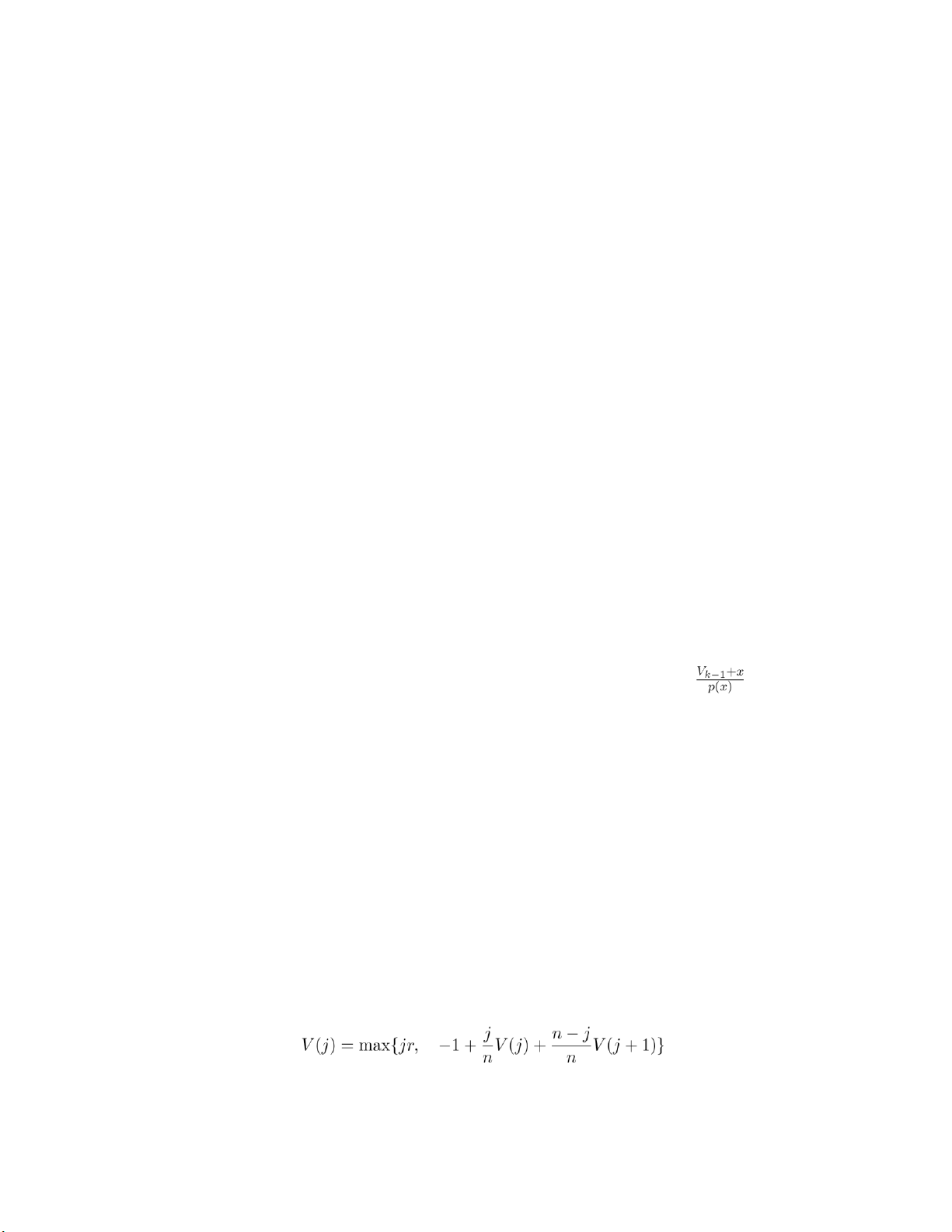
12.4 The optimal policy is to accept any offer i such that
i(1 − β) ≥ β(E[(X − i)+ − c)
12.5 (a) Before you can get to k in a row you must have k − 1. So the optimal policy when you need
k in a row is to get to k − 1 in a row at minimal expected cost and then invest some amount x in the next game. (b)
If you invest xin the next game after you have reached k − 1 in a row at minimal expected
cost, then the number of times you will get to k − 1 in a row is geometric with parameter p(x).
Hence, as the expected cost to get to k − 1 in a row is Vk−1, your expected cost . (c)
Once Vn is determined, we find the optimal policy as follows. Let H(j) be the minimal
expected additional cost to get to n wins in a row when you currently have j consecutive wins.
Then H(j) = min{x + p(x)H(j + 1) + (1 − p(x))Vn}, j < n. x
Starting with j = n − 1, then j = n − 2, the preceding can be recursively solved for. The x that
mininizes the right side of the preceding equation is the optimal amount to invest when you
currently have j wins in a row.
12.6 (a) The state is the number of distinct type in the current collection. The action is whether to
stop or to collect another coupon.
(b) With V (j) equal to the maximal expected additional return if one currently has j distinct types, the optimality equation is
(c) Theone-stage lookahead policy stops in state j if 27 lOMoARcPSD|359 747 69 That is, it stops in state .
(d) It is optimal because, as the state cannot decrease, its set of stopping states is closed.
(e) The state is the subset of types in cone’s collection. (d) If S is the subset of types, then the one-
stage lookahead policy stops if r Xpi ≤ 1. i/∈S
It is optimal because the set of coupons in one’s collection is one continues must always include
what is currently in one’s collection.
12.7 The one-stage lookahead policy would stop whenever the number of red balls is less than or
equal to the number of black balls. It is a very bad policy. 28 lOMoARcPSD|359 747 69
13.1 Assume u ≤ r. Let s be the price of the security at time y, where y < t. If, rather than exercising
at time y < t, we exercised at time t (regardless of the price at time t) then the expected time y return is
e−r(t−y)(ser(t−y) − Keut) = s − Keut−r(t−y) ≥ s − Keuy
The result follows because the right hand side is the time y return if we exercise at time y.
13.3 Solution given in text. 13.4 n n Var(W) =
Cov(Y + XciXi, Y + XcjXj) i=1 n n =
Cov(Y,Y ) + 2Cov(Y,XcjXj) + Cov(XciXi, XcjXj) j=1j=1 n =
Var(Y ) + 2XciCov(Y,Xi) + XXcicjCov(Xi,Xj) n =
Var(Y ) + 2XciCov(Y,Xi) + Xc2i Cov(Xi,Xi) + XXcicjCov(Xi,Xj)
i=1 j=6 i =
Var(Y ) + 2XciCov(Y,Xi) + Xc2i Var(Xi) i=1 i=1
where the final equality used the independence of Xi,Xj to conclude that, for i =6 j, Cov(Xi,Xj) = 0.
(c) Setting the partial derivative of the preceding with respect to ci equal to 0 gives the result:
2ciVar(Xi) + 2Cov(Y,Xi) = 0 29 lOMoARcPSD|359 747 69
13.7 Similar to what is done in Section 11.8 except we now let
Vk(i) = max{suidk−i − K,
pVk+1(i + 1) + (1 − p)Wk+1(i)}
13.8 The price is either multiplied by u with probability p or by d with probability 1−p, and if
multiplied by d we need to check if the new price is an end of day price that is below the barrier. 30 lOMoARcPSD|359 747 69 Solutions Manual to
AN INTRODUCTION TO MATHEMATICAL
FINANCE: OPTIONS AND OTHER TOPICS Sheldon M. Ross 1.1 1.2 1.3 1.4 1.5
1. The probability that their child will develop cystic fibrosis is the probability thatthe
child receives a CF gene from each of his parents, which is 1/4.
2. Given that his sibling died of the disease, each of the parents much have exactlyone
CF gene. Let A denote the event that he possesses one CF gene and B that he does
not have the disease (since he is 30 years old). Then
1.6 Let A be the event that they are both aces and B the event they are of different suits. Then 1.7
Part (b) follows from part (a) since from (a) A and Bc are independent, implying from (a)
that so are Ac and Bc. lOMoARcPSD|359 747 69 1
1.8 If the gambler loses both the bets, then X = −3. If he wins the first bet, or loses the
first bet and wins the second bet, X = 1. Therefore, 1. 2. 1.9
1. E[X] is larger since a bus with more students is more likely to be chosen than a bus with less students. 2.
1.10 Let N denote the number of sets played. Then it is clear that P{N = 2} = P N
1.11 Let µ = E[X].
1.12 Let F be her fee if she takes the fixed amount and X when she takes the contingency amount.
E[F] = 5,000, SD(F) = 0
E[X] = 25,000(.3) + 0(.7) = 7,500 lOMoARcPSD|359 747 69 2
E[X2] = (25,000)2(.3) + 0(.7) = 1.875 × 10⁸ Therefore, 1.13 ] = 1.14 Cov(X,Y ) = = = = 1.15 lOMoARcPSD|359 747 69 3 (b) Cov(X,X) =
E[(X − E[X])2] = Var(X) (d) Cov(c,Y ) =
E [(c − E[c])(Y − E[Y ])] = 0 1.16
Cov(aU + bV,cU + dV ) =
Cov(aU,cU + dV ) + Cov(bV,cU + dV ) =
Cov(aU,cU) + Cov(aU,dV ) + Cov(bV,cU) + Cov(bV,dV )
= ac(1) + ad(0) + bc(0) + bd(1) = ac + bd
1.17 With c(i,j) = Cov(Xi,Xj)
(a) c(1,3) + c(1,4) + c(2,3) + c(2,4) = 21
(b) 2 + 3 + 4 + 4 + 6 + 8 + 6 + 9 + 12 = 54 1.17
Let Xi be the amount it goes up in period i. Then and
Cov(X1,Y ) = Cov(X1,X1) = Var(X1) = 1/4 Therefore, Corr( 1.18
No, since for such a pair Corr(X,Y ) = 2, and correlations are always between −1 and 1. 2.1
1. P(Z < −.66) = P(Z > .66) = 1 − P(Z < .66) = 1 − Φ(.66) = 1 − .7454 = .2546 2.
P(|Z| < 1.64) =
P(Z < 1.64) − P(Z < −1.64) =
P(Z < 1.64) − [1 − P(Z < 1.64)]
= 2Φ(1.64) − 1 = 2 × .9495 − 1 = .8990
3. P(|Z| > 2.20) = 2P(Z > 2.20) = 2[1 − P(Z < 2.20)] = 2(1 − .9861) = .0278 2.2 x = 2 lOMoARcPSD|359 747 69 4 2.3
P(|Z| > x) = P(Z > x or Z < −x) = P(Z > x) + P(Z < −x) = 2P(Z > x)
where the last equality comes from the fact that Z is symmetric.
2.4 a = 2µ, b = −1.
Cov(X,Y ) = −Var(X) = −σ2 2.5
(a) 127.7 ± 19.2
(b) 127.7 ± (1.96)(19.2)
(c) 127.7 ± 57.6
2.6 Let X1 and X2 denote the life of the first and the second battery respectively. It is
given that X1 and X2 are both normal random variables with mean 400 and standard
deviation 50. Let Z denote a standard normal random variable.
1. X1 +X2 is a normal random variable with mean 800 and standard deviation 50
2. X2 − X1 is a normal random variable with mean 0 and standard deviation 50
3. P(|X1 − X2| > 25) = 2P(X2 − X1 > 25) ≈ .7236
2.7 Let Xi be the time the that it takes to develop the ith print. Then, the time that
it takes to develop 100 prints, call it X, can be expressed as
It follows from the central limit theorem that X approximately has a normal distribution
with mean 1800 and standard deviation 10. Therefore, lOMoARcPSD|359 747 69 5
The probability for part (b) is 0
2.8 Let Xi be the mileage for person i, i = 1,...,30. From central limit theorem,
is approximately a normal random variable with mean 25000× 30 and standard deviation 12000 1. 2.
2.9 Let Si be the price of stock in time period i. Then Si+1 = SiXi where the random
variable Xi is defined as
u ,with probability p
d ,with probability 1 p Xi = ( − Then lOMoARcPSD|359 747 69 6
We can use the central limit theorem to approximate with a normal random
variable Y with the same mean and variance. E[Y ] = Var(Y ) =
= 1000 (p(logu)2 + (1 − p)(logd)2 − .00137872) ≈ 0.1206 Therefore
where Z stands for a standard normal random variable.
2.10 Let Xi be the movement in period i. Then we can approximate with a
normal random variable Y with the same mean and variance 700 · E[Y ] =
EXXi¸ = 700(−.39 + .41) = 14 i=1 700 µ Var(Y ) =
VarXXi¶ = 700(.39 × 1.022
+ .20 × .022 + .41
× .982) = 559.72 i=1 Therefore, 3.1
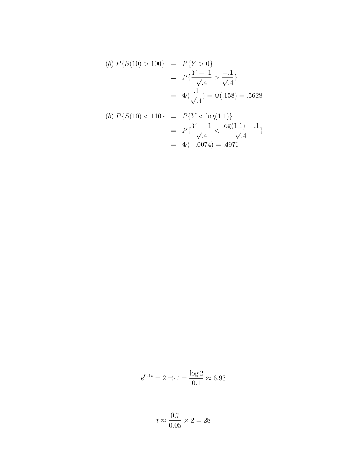
(a) 100e.1+.2 = 100e.3
For parts (b) and (c), use that Y ≡ log(S(10)/100) is normal with mean .1 and variance .4. This gives lOMoARcPSD|359 747 69 7
3.4 Since S(t)/S(0) is distributed as eX when X is normal with mean µt and variance tσ2, it follows that
E[S(t)/S(0)] = E[eX] = eµt+tσ2/2
3.5 Using the representation in problem 3.4, we obtain
E[S2(t)/S2(0)] = E[e2X] = e2µt+2tσ2
where the preceding used that 2X is normal with mean 2µt and variance 4tσ2. Therefore,
Var(S(t)) = E[S2(t)] −2 (E[S(t)])2
= s20e2µt+2tσ2 − 2s20e2µt+tσ2
= s20e2µt+tσ (etσ − 1) 4.1
(a) re = (1 + 0.1/2)2 − 1 = 0.1025
(b) re = (1 + 0.1/4)4 − 1 ≈ 0.1038
(c) re = e0.1 − 1 ≈ 0.1052
4.2 Suppose it takes t years to double, then
4.3 Suppose it takes t years to quadruple, then we can solve t from 1.05t = 4. We
can also use the doulbing rule to approximate t, which gives lOMoARcPSD|359 747 69 8
If the interest is 4%, then it is approximately 0.7/0.04 × 2 = 35 years.
4.4 Using that er ≈ 1+r, when r is small, we see that if (1+r)n = 3 then enr ≈ 3. Thus,
4.5 Suppose you need to invest x at the beginning of each of the next 60 months
to have a value of $100,000 at the end of 60 months, then Solve to get
4.6 Let’s compute the present value, denoted by S, of this cash flow.
Since it is negative, it is not worth investing.
4.7 (15 pts) Let the present value of the first cash flow sequence be S1 and that
of the second cash flow sequence be S2. Then
(a) r = 0.03, S1 = 82.71,S2 = 84.63. The second one is preferable. (b) r =
0.05, S1 = 78.37,S2 = 78.60. The second one is preferable.
(c) r = 0.1, S1 = 69.01,S2 = 65.99. The first one is preferable.
4.8 (15 pts) Let S denote the present value, then
(b) r = 0.10, S = 0.
(c) r = 0.12, S = −736.01.
4.9 The effective interest rate, call it r, is that value for which lOMoARcPSD|359 747 69 9 which reduces to
Solution by trial and error shows that r ≈ .015. That is, the effective interest rate is 1.5 percent per month. 4.11
The cost-flow sequences are as follows
buy at beginning of year 1: 22 7 8 9 10 -4 buy at
beginning of year 2: 9 25 7 8 9 -9 buy at beginning of year 3: 9 11 28 7 8 -14
buy at beginning of year 4: 9 11 13 31 7 -19
With the yearly interest rate 10%, the present value of the first cost-flow sequence is
Similarly, the prevent values of the other three cost-flow sequences can be determined,
and the four present values are
46.08, 44.08, 44.17, 46.02
Therefore, the company should purchase a new machine one year from now. 4.12
Since the bank charges 2 points, the amount of money we receive for
this loan is actually 120,000 × 0.98 = 117,600. The interest we need to pay per month is 120,000 ×
0.5% = 600. Therefore the cash flow sequence of this loan is time (mths) 0 1 2 ... 35 36 cash flow
117600 -600 -600 ... -600 -120600
Let r be the effective interest rate per month for this loan, then
We can solve the above to get r ≈ 0.5615%. 4.13
The present value of paying the entire amount of $16,000 now is
simply $16,000, while the present value of paying $10,000 now and another
$10,000 at the end of ten years is
S = 10,000 + 10,000(e−r)10 lOMoARcPSD|359 747 69 10 Therefore
(a) r = 0.02, S = 18,187.31, which is not preferable. (b) r
= 0.05, S = 16,065.31, which is not preferable.
(c) r = 0.10, S = 13,678.79, which is preferable.
4.14 The cash flow sequence is as follows,
time (yrs) 0 0.5 1 ... 4.5 5 cash flow -1000 30 30 ... 30 1030
With a continuously compounded interest 5%, the present value of above is
4.15 The present value of a cash flow of 1,000 at the end of 10 years with a
continuously compounded interest rate 8% is
4.16 The rate of return is the effective interest rate which makes the present value of
the cash flow streams equal to the initial payment. Therefore (a)
Take 1 + r as the variable and use the formula to solve the above, we get
Since 1 + r can not be negative, so 1 +
(b) In this case, it is easy to see that r = 0. (c) Similar to part (a), 4.18 lOMoARcPSD|359 747 69 11 942%
4.20 Since the interest rates for borrowing and lending are not the same, we can not
compute the present value of the whole cash flow stream by summing up the present
values of each item as we did before. For example, when we receive $900 a year from
today, we will choose to use that money paying off part of the debt rather than earning
interest on it. So, let’s start by borrowing $1000 and examine our balance year by year. time account balance
today−10001000 ×11.08 + 800 = 605.08 + 900 = −180.6
end of year 1end of year 3 −180 × 1.05 −08 +
700 = 901200 = −564.7504.12 end of year 2
−605.6 ×12 × 1. end of year 4 −564.
This means that if you start with nothing, this investment gives you $90.7504 four years
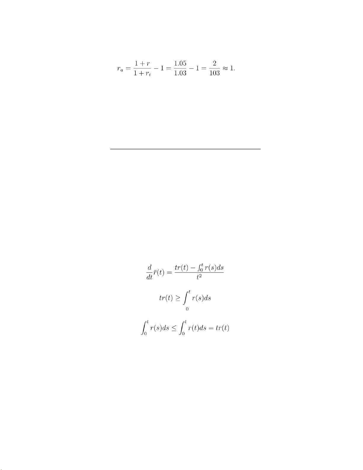
from today. Therefore,you should invest. 4.21 Thus, we must show that which follows since 4.22 Note that
P(αt) = e−αtr¯(αt), Pα(t) = e−αtr¯(t) Hence, P(αt) ≥
Pα(t) is equivalent to ¯r(αt) ≤ r¯(t). lOMoARcPSD|359 747 69 12
5.2 Let s be the price of the stock today and r the one period simple interest rate.
Suppose that we buy x shares of call options and y shares of stocks today, then since
K < minsi, the call option will be exercised after one period in all cases. Therefore,
the value of our holdings at time 1 is x(si − K) + ysi if the stock price at time 1 is si. If
we choose x = −y, then we have a riskless return of −xK. To rule out an arbitrage
opportunity, this riskless return should be equal to Therefore
5.3 Let K denote the strike price of the call and t the expiration date. Also, let
S(t) be the price of the stock when the call expires. Then the value of the call at time t is
vc = max{0,S(t) − K}
and the value of the stock at time t is
vs = S(t)
It is clear that vs ≥ vc since K ≥ 0. Therefore one share of stock is preferred to one share of
call option, which leads to the conclusion that C ≤ S.
We can also do this by arguing that an arbitrage opportunity exists if C > S. In this case,
one can buy one share of stock and sell a call option today, which gives C − S dollars. When
the call option expires, the value of the portfolio is
vs − vc = min{S(t),K} > 0 Therefore it is an arbitrage.
5.4 (a) is not true. (b) is true. The easiest way to see this is to use the put call
parity and the result from Exercise 5.3.
P − Ke−rt = C − S ≤ 0 Therefore
P ≤ Ke−rt ≤ K
Also, one can argue that an arbitrage opportunity exists if P > K. lOMoARcPSD|359 747 69 13
5.5 From the put call parity,
P − Ke−rt + S = C ≥ 0 Therefore
P ≥ Ke−rt − S
Also, one can argue that an arbitrage opportunity exists if the inequality doesn’t hold.
5.7 Let P(t) denote the price of an American put option having exercise time t.
Given s < t, we want to show that P(s) ≤ P(t).
We prove this by showing that an arbitrage is present if the statement is not true.
Suppose P(s) > P(t), then we buy one share of the put option having exercise time t and
sell one share of the put option having exercise time s, which gives us P(s) − P(t) dollars
today. Consider the strategy that whenever the put option we sold is exercised by the
buyer, we exercise our put option at the same time. This strategy guarantees us no cash
flow in the time period (0,s]. On the other hand, if the put option we sold is not exercised
by the buyer, we then still have our put option at time s, whose value is always nonnegative.
Either way, it is a sure win situation (remember we receive P(s) − P(t) today), therefore an arbitrage.
5.8 No, it is not valid for European puts. Suppose we buy the put option having
exercise time t and sell the put option having exercise time s, where s < t. If the sold
put option is exercised at time s, we are forced to pay K for one share of stock. At
time t, we have a debt of Ker(t−s) and our put option guarantees us to sell that stock
for at least K, which is not enough to pay off the debt. Therefore, we can not guarantee a sure win.
5.9 s − d 5.10
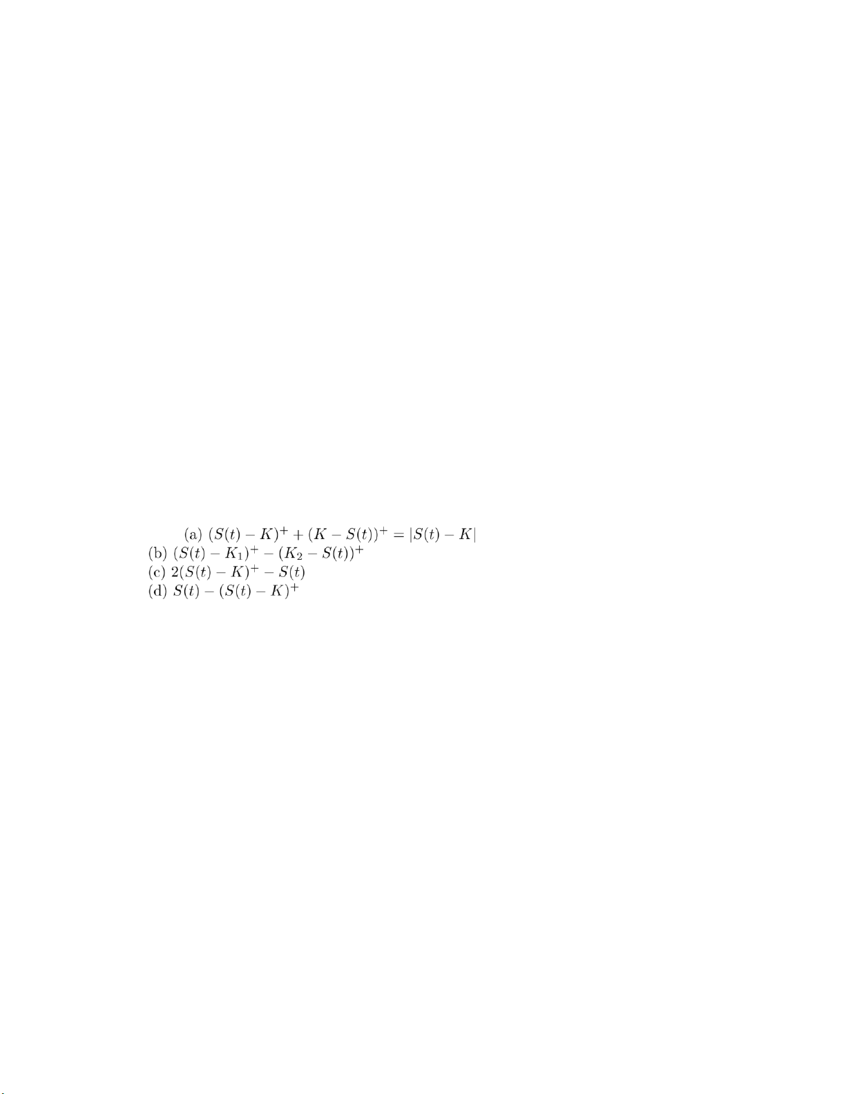
(a) If S(t) > K, the call option is worth S(t) − K and the put option is worthless. On the
other hand if S(t) < K, the put option is worth K −S(t) and the call option is worthless.
Therefore, the payoff is |S(t) − K|.
(b) Consider the following two cases. K1 ≥ K2, then
,S(t) > K1
payoff =,K2 ≤ S(t) ≤ K1
,S(t) < K2
K1 < K2, then lOMoARcPSD|359 747 69 14
,S(t) > K2
payoff =,K1 ≤ S(t) ≤ K2
,S(t) < K1
5.7 Let P(t) denote the price of an American put option having exercise time t.
Given s < t, we want to show that P(s) ≤ P(t).
We prove this by showing that an arbitrage is present if the statement is not true.
Suppose P(s) > P(t), then we buy one share of the put option having exercise time t and
sell one share of the put option having exercise time s, which gives us P(s) − P(t) dollars
today. Consider the strategy that whenever the put option we sold is exercised by the
buyer, we exercise our put option at the same time. This strategy guarantees us no cash
flow in the time period (0,s]. On the other hand, if the put option we sold is not exercised
by the buyer, we then still have our put option at time s, whose value is always nonnegative.
Either way, it is a sure win situation (remember we receive P(s) − P(t) today), therefore an arbitrage.
5.8 No, it is not valid for European puts. Suppose we buy the put option having
exercise time t and sell the put option having exercise time s, where s < t. If the sold
put option is exercised at time s, we are forced to pay K for one share of stock. At
time t, we have a debt of Ker(t−s) and our put option guarantees us to sell that stock
for at least K, which is not enough to pay off the debt. Therefore, we can not
guarantee a sure win. 5.10
(a) If S(t) > K, the call option is worth S(t) − K and the put option is worthless. On the
other hand if S(t) < K, the put option is worth K −S(t) and the call option is worthless.
Therefore, the payoff is |S(t) − K|.
(b) Consider the following two cases. K1 ≥ K2, then
S(t) − K1
,S(t) > K1 payoff = 0
S(t) − K2
,S(t) < K2 ,K2
K1 < K2, then ≤ S(t) ≤ K1 lOMoARcPSD|359 747 69 15
,S(t) > K2
payoff =,K1 ≤ S(t) ≤ K2
,S(t) < K1 6.1
We need to see whether we can find a probability vector (p1,p2,p3) for which
all bets are fair. In order to have all bets fair, pi = 1/(1 + oi). Therefore, p1 = 1/2 p2 = 1/3 p3 = 1/6
Since the pi’s sum up to 1, (p1,p2,p3) is indeed a probability vector which makes all bets fair.
Therefore, no arbitrage is present. 6.2
To rule out the arbitrage opportunity, o4 must satisfy the equation,
Therefore, o4 = 47/13. 6.3 No arbitrage is present since 6.4
If no arbitrage is present, then (p1,p2,p3) = (1/2,1/3,1/6) has to be the
probability vector which makes all bets fair. Therefore
o12(p1 + p2) − p3 = 0 ⇒ o12 = 1/5
o23(p2 + p3) − p1 = 0 ⇒ o23 = 1
o13(p1 + p3) − p2 = 0 ⇒ o 13 = 1/2 6.5
If the outcome is j, then the betting scheme xi,i = 1,...,m, gives me 6.6
From Example 6.1b, p = (1+2r)/3. The payoff of the put option is 0 if the
stock price goes up, and 100 if the stock price goes down. To rule out arbitrage, the
expected return of buying one put option under the probability distribution has to be zero. That is, Therefore lOMoARcPSD|359 747 69 16 The put-call parity says
In this example, one can check the following indeed holds. 6.7
Since the call option expires in period 2 and the strike price K = 150, it is clear that Cuu = 250 Cud = 0 Cdd = 0
Let p denote the risk neutral probability that the price of the security goes up, then
where we assume r = 0. Then we can find C by computing the expected return of the call
option in the risk neutral world. 6.8 See Example 8.1a for details. 6.9
We need to find a betting strategy which gives a weak arbitrage if (a) C = 0
and (b) C = 50/3.
(a) C = 0. In this case it is clear that buying one share of stock is a weak arbitrage. At
time 0, one does not have to pay out anything. At time 1, the profit is 50 if the stock
goes up to 200, and 0 if the stock price is either 100 or 50.
(b) C = 50/3. In this case it is not that clear how a weak arbitrage can be established.
But since the price of the call option is high, it’s intuitive that we want to sell it. So,
let’s consider a portfolio consisting of selling one share of the call option and buying
x share(s) of the stock. Our return depends on the price of stock at time 1, which is tabulated as follows. lOMoARcPSD|359 747 69 stock balance value of the portfolio profit price at time 1 at time 0 at time 1 (r = 0) 17 200 50/3 − 100x −50 + 200x 100x − 100/3 − 100 50/3 − 100x 0 + 100x 50/3 − 50 50/3 100x 0 + 50x 50x + 50/3
From the above table, if we choose x = 1/3, then the profit is 50/3 if the stock price
is 100 at time 1, and 0 otherwise, which is a weak arbitrage. 7.1 7.2
Since the unit of time is one year, t = 4/12 = 1/3. The probability that the
call option will be exercised at t = 1/3 is the probability that the stock price at t = 1/3 is
greater than the strike price K = 42, which is
where X is a normal random variable with mean µt = .12/3 = .04 and standard deviation
σ√t = .24/√3. Therefore, the above probability is equal to 7.3 The parameters are t = 1/3 r = .08 σ = .24 K = 42 S = 40 so we have that Therefore,
7.4 From the put-call parity, we can derive the no-arbitrage cost to a put option
where ω is defined in equation (7.7) in text (page 87). The parameters are K = 100 S(0) = 105 r = .1 σ = .30 t = 1/2 lOMoARcPSD|359 747 69 18 Therefore,
P = 105(.7163 − 1) + 100e−.05(1 − .6404) ≈ 4.418 7.5
A call option with a strike price equal to zero is equivalent to a stock, since
the payoff is max{0,S(t)−K} = max{0,S(t)−0} = S(t). Therefore, the price of such a call
option is equal to the price of the stock S(0).
The same conclusion can be easily verified by the B-S formula by plugging in K = 0. 7.6
From the Black-Scholes formula, ω → ∞ as t → ∞. Therefore, as t → ∞,
C = S(0)Φ(ω) − Ke−rtΦ(ω − σ√t) → S(0) × 1 − K × 0 = S(0)
7.7 The payoff is F if S(t) > K and 0 otherwise. So, the risk-neutral valuation (or the
unique no-arbitrage cost) of such a call is equal to
Ca = e−rtF × P{S(0)eW > K}
where W is normal with mean (r−σ2/2)t and variance σ2t (see page 88 in text). Therefore
where Z stands for a standard normal random variable and
as defined in equation (7.7) in text (page 87). The parameters F = 100 K = 40 S(0) = 38 σ = .32 r = .06 t = 1/2 So Therefore, lOMoARcPSD|359 747 69 19
8.1 If there is no arbitrage, then there exists p = (p50,p175,p200) such that both buying
stocks and buying call options are fair. This means we are able to solve (p50,p175,p200) from
the following linear equations.
−C + 25p175 + 50p200 = 0 (0.1)
−50p50 + 75p175 + 100p200 = 0 p50 (0.2)
+ p175 + p200 = 1 (0.3)
0 ≤ p50,p175,p200 ≤ 1 (0.4)
By letting p50 = x, we can solve p175 and p200 in terms of x from (2) and (3), which gives p175 = 4 − 6x p200 = 5x − 3
Together with the constraint in (4), the solution from (2)–(4) can be written as
(p50,p175,p200) = (x,4 − 6x,5x − 3)
3/5 ≤ x ≤ 2/3
Therefore, if C = 25p175 + 50p200 = 100x − 50 where 3/5 ≤ x ≤ 2/3, then we are able to solve
the linear equations (1)–(4). In other words, if 10 ≤ C ≤ 50/3, there is no arbitrage opportunity. 8.2 (a)
u(x) = logx
u′(x) = 1/x
u′′(x) = −1/x2
Therefore a(x) = 1/x. (b)
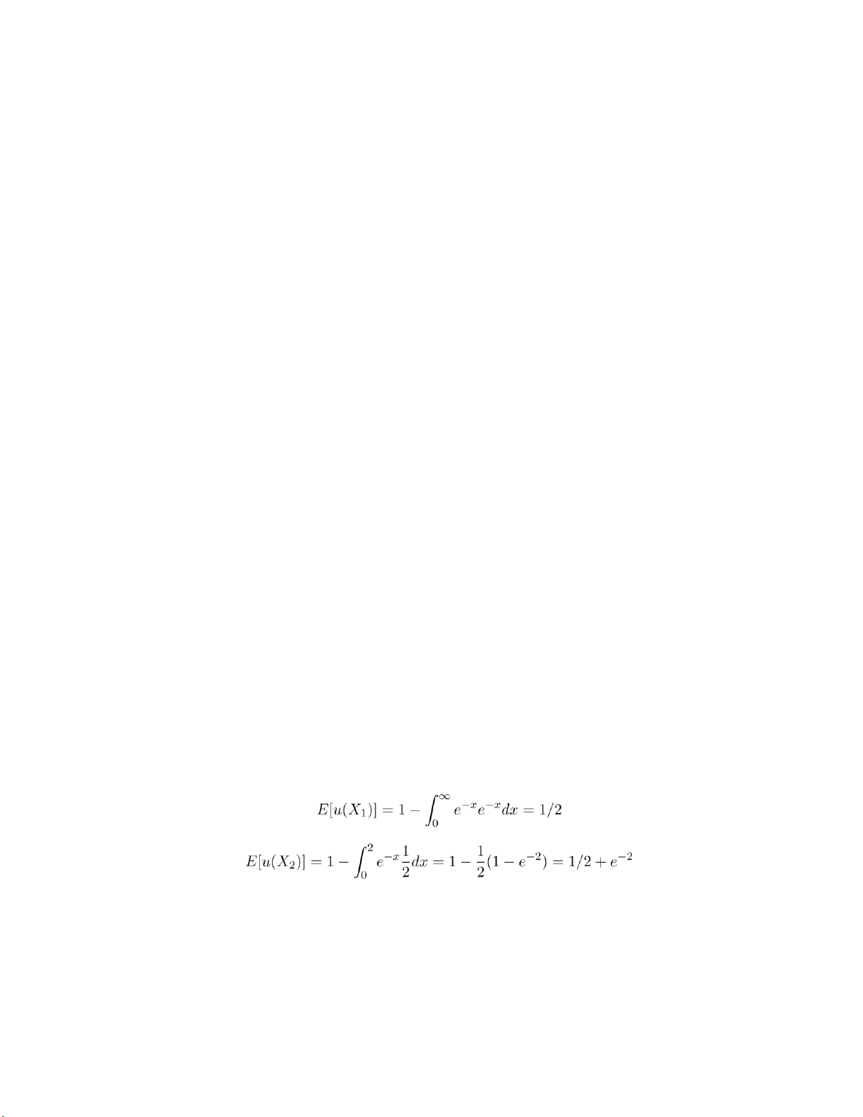
u(x) = 1 − e−x
u′(x) = e−x
u′′(x) = −e−x
Therefore a(x) = 1.
8.3 Using the notation defined in Example 8.2a, let f(α) denote the expected utility of the final fortune, then −
Since p < 1/2, f′(α) < 0 for 0 ≤ α ≤ 1, the maximum value of f(α) for 0 ≤ α ≤ 1 is obtained at α = 0.
8.7 Using the notation on page 117,
where w is the initial wealth, αi is the proportion of the initial wealth invested in security
i, and Xi is the return from security i if the initial investment is $1. If U(x) = logx, then lOMoARcPSD|359 747 69 20 n · µ
E[U(W)] = E[log(W)] =
Elogw XαiXi¶¸ i=1 n · µ =
Elogw + logXαiXi¶¸ i=1 n · µ = logw + ElogXαiXi¶¸
i=1 So, the optimal αi,i = 1,...,n do not depend on w.
8.8 To show that the second derivative is nondecreasing, we need to show that the
third derivative is nonnegative.
(a) For 0 < a < 1,
U′(x) = axa−1
U′′(x) = a(a − 1)xa−2
U′′′(x) = a(a − 1)(a − 2)xa−3 > 0
(b) U′(x) = be−bx, U′′(x) = −b2e−bx, so U′′′(x) = b3e−bx > 0.
(c) U′(x) = x−1, U′′(x) = −x−2, so U′′′(x) = 2x−3 > 0.
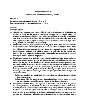
8.11 The objective is to maximize the probability that W > g, or
where Z stands for a standard normal random variable. Therefore, to maximize the
probability, it is equivalent to minimize or to maximize
Document Outline
- 2.
- 1. P(Z < −.66) = P(Z > .66) = 1 − P(Z < .66) = 1 − Φ(.66) = 1 − .7454 = .2546
- P(|Z| < 1.64) = P(Z < 1.64) − P(Z < −1.64)
- 2.3
- where the last equality comes from the fact that Z is symmetric. 2.4 a = 2µ, b = −1. Cov(X,Y ) = −Var(X) = −σ2
- (c) 127.7 ± 57.6
Tài liệu liên quan:
-

Syllabus Môn Finance - Banking | Trường Đại học Quốc tế, Đại học Quốc gia Thành phố Hồ Chí Minh
109 55 -
Answers Questions and Practice problems Chapter 17 | Môn Finance - Banking - Trường Đại học Quốc tế, Đại học Quốc gia Thành phố Hồ Chí Minh
102 51 -
Solution Stocks Môn Finance - Banking | Trường Đại học Quốc tế, Đại học Quốc gia Thành phố Hồ Chí Minh
117 59 -
What is Behavioral Finance | Môn Finance - Banking - Trường Đại học Quốc tế, Đại học Quốc gia Thành phố Hồ Chí Minh
110 55 -
Loan Analysis & Futures | Môn Finance - Banking - Trường Đại học Quốc tế, Đại học Quốc gia Thành phố Hồ Chí Minh
101 51