Statictic assignment - Statistics for Business | Trường Đại học Quốc tế, Đại học Quốc gia Thành phố HCM
Statictic assignment - Statistics for Business | Trường Đại học Quốc tế, Đại học Quốc gia Thành phố HCM được sưu tầm và soạn thảo dưới dạng file PDF để gửi tới các bạn sinh viên cùng tham khảo, ôn tập đầy đủ kiến thức, chuẩn bị cho các buổi học thật tốt. Mời bạn đọc đón xem!
Môn: Statistics for Business (BAO8OIU) 43 tài liệu
Trường: Trường Đại học Quốc tế, Đại học Quốc gia Thành phố Hồ Chí Minh 1.9 K tài liệu
Tác giả:


Preview text:
Vũ Minh Ngọc – MSSV: BABANS21128
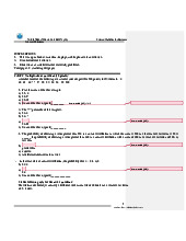
Monday – Morning – Lession 4-5-6 – Room A1.201 ASSIGNMENT 1 1.
Yes, because the statement doesn’t show enough information, it doesn’t make sense or
connect to the causes. Moreover, if the statement is true and it may have some evidence, it
is still research from a sample, which means that a small group holds no matter. 2. a)
- Choose randomly 10 moviegoers by using =RANDBETWEEN(bottom, top), each person
has the same change of being chosen( allow duplicates) 32 34 33 12 57 13 58 16 23 23 62 65 35 15 17 20 14 11 51 33 31 13 11 58 23 10 63 34 12 15 62 13 40 11 18 62 64 30 42 20 simple random sampling (the ages of moviegoers) 58 63 33 12 35 40 23 23 57 58 b) 32 34 33 12 57 13 58 16 23 23 62 65 35 15 17 20 14 11 51 33 31 13 11 58 23 10 63 34 12 15 62 13 40 11 18 62 64 30 42 20 21 56 11 51 38 49 15 21 Systematic sampling samples total(N) periodicity start (n) 10 48 5 11 11 51 38 49 15 11 58 23 10 63
- Calculate the periodicity by N/n = 5, starting at 11, sample every 5 items to obtain
a sample of n=10 items from a list of N=48 items. c)
The proportion of all 48 moviegoers who were under age 30 is 0,5.
+ Use COUNTIF function to count the number of moviegoers who were under 30
(24 people) then devide by 48, we got the proportion 0,5 or 50% of moviegoers were under age 30. d) 23 62 34 51 56 23 30 49 11 17 moviegoers were under age 4 30 proportion 0.4 63 56 51 21 14 40 58 23 57 21 moviegoers were under age 4 30 proportion 0.4 14 12 15 62 11 56 42 23 56 33 moviegoers were under age 5 30 proportion 0.5
e) Through each sample , we can see that the sample proportion are close to the population proportion 3.
a. the population of interest to the university administration: university’s students
b. the sample of interest to the university administration: 250 students
c. the variable of interest to the university administration: the average parking time of the students 4.
a. population of interest: computer chips b. sample: 1000 chips
c. parameter: proportion of defective products
d. statistic: proportion of a sample chips which is defective
e. the value 10% refer to the parameter
f. the value 7.5% refer to the statistic
g. Because statistic is a set of data drawn from the population, so we pick randomly a
number of observations, from this sample we can calculate, study and drawn the conclusion.
- From the statement above, we can conclude that the claim is true because the statistic(
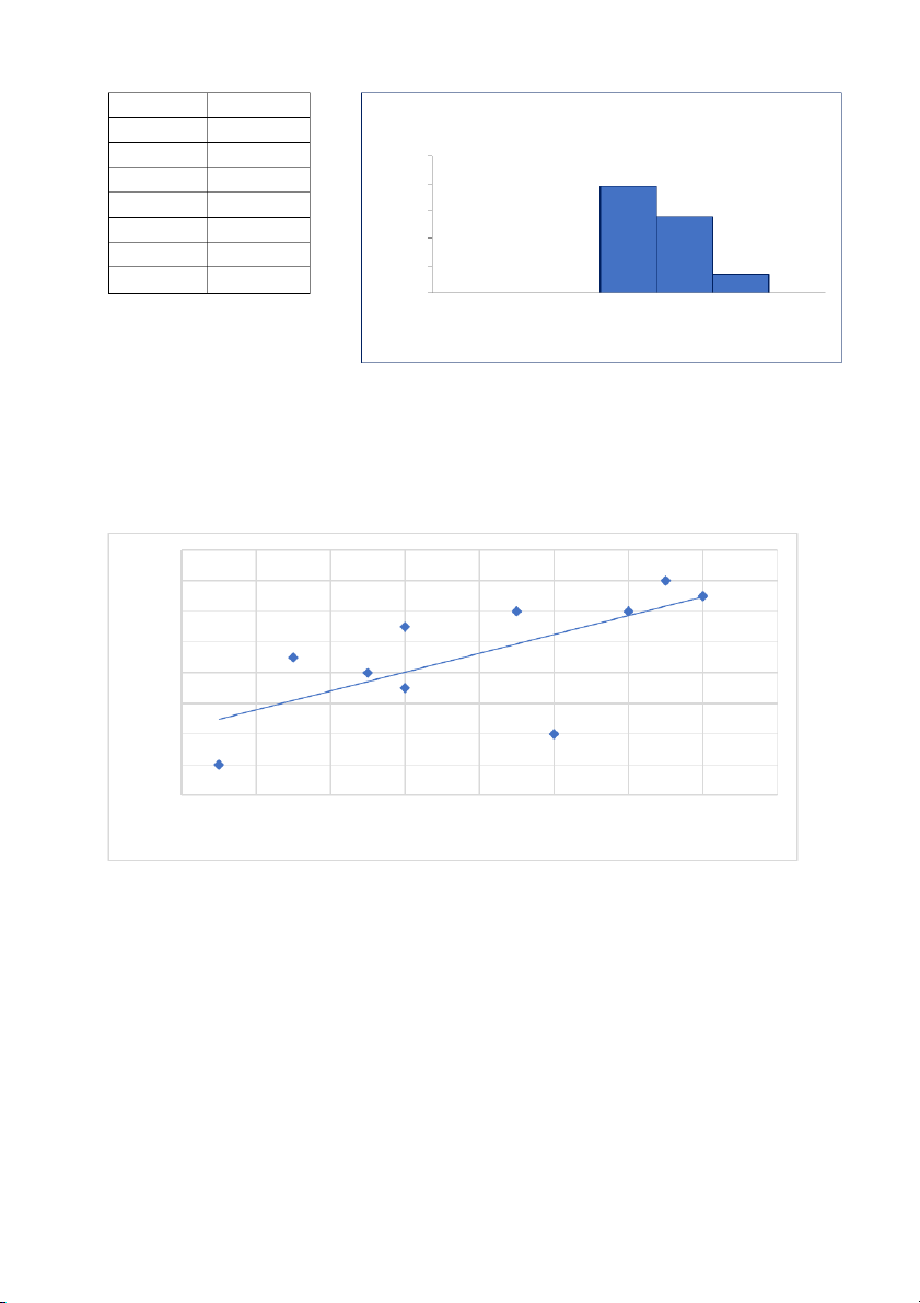
the sample proportion) is less than 10% (7.5%) 5. a. - number of bins: 74
- bin limits: k = 1 + 3.3log(n) = 7.2 6.54 6.58 6.58 6.62 6.66 6.7 6.71 6.73 6.75 6.75 6.76 6.76 6.76 6.77 6.77 6.79 6.81 6.81 6.82 6.84 6.85 6.89 6.9 6.91 6.91 6.92 6.93 6.93 6.94 6.95 6.95 6.95 6.96 6.96 6.98 6.99 7 7 7 7.02 7.03 7.03 7.03 7.04 7.05 7.05 7.07 7.07 7.08 7.11 7.11 7.13 7.13 7.16 7.17 7.18 7.21 7.25 7.28 7.28 7.3 7.33 7.33 7.35 7.37 7.38 7.45 7.56 7.57 7.58 7.64 7.65 7.87 7.97 bins 8 Lower Upper bin width 0.5 5 5.5 5.5 6 6 6.5 n 74 6.5 7 7 7.5 7.5 8 Bin Frequency Histogram 5.5 0 6 0 50 6.5 0 40 7 39 30 7.5 28 20 requency 8 7 F 10 More 0 0 5.5 6 6.5 7 7.5 8 More Bin Shape: Right Skewed 6. 450 400 350 300 250 SAVINGS 200 150 100 50 0 1 2 3 4 5 6 7 8 TIMES ( HOURS)
As we can see in the chart, the line goes up so, we can conclude that in general, people who
spend more time can save more money. 7. a. b. The monthly unemployment The monthly unemployment rate rate 8 8 7.5 6 te te a 7 a 4 R R 6.5 2 6 0 1 2 3 4 5 6 7 8 9 10 11 12 1 2 3 4 5 6 7 8 9 10 11 12 Month Month c.
- As we can see in the two bar chart below, the A bar chart shows the distribution more
clearly because the columns are more distinct. The B bar chart still shows the full data but
makes the data generally not much different. d.
- I will use the A bar chart as the reason I have showed below, the A bar chart illustrates
the data more clearly, so we can compare data between months more easily and accurately. 8.
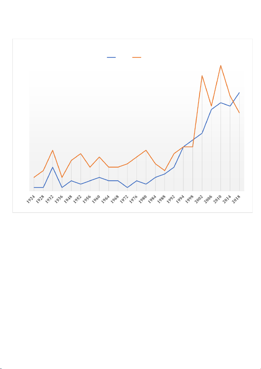
Total number of medals won at the Winter Olympics 40 Canada United States 35 30 25 S L A 20 D E M 15 10 5 0 YEAR
The US almost always wins more medals than Canada, but from the line chart below, we
can see that the number of medals won by the US has fluctuated year by year.
Meanwhile, the number of medals that Canada has achieved witnessed an erratic growth
and always keeps around 5 medals. Until 1994, the number of medals achieved began to
increase gradually and reached 29 medals in 2018, 6 more than the US.
Tài liệu liên quan:
-
Đề thi giữa kỳ học phần Statistics for Business năm 2015 | Trường Đại học Quốc tế, Đại học Quốc gia Thành phố Hồ Chí Minh
323 162 -
Đề thi giữa kỳ học phần Statistics for Business có đáp án | Trường Đại học Quốc tế, Đại học Quốc gia Thành phố Hồ Chí Minh
385 193 -
Đề thi giữa kỳ học phần Statistics for Business năm 2019 | Trường Đại học Quốc tế, Đại học Quốc gia Thành phố Hồ Chí Minh
270 135 -
Đề thi giữa kỳ học phần Statistics for Business | Trường Đại học Quốc tế, Đại học Quốc gia Thành phố Hồ Chí Minh
283 142 -
Bài tập tiểu luận nhóm học phần Statistics for Business | Trường Đại học Quốc tế, Đại học Quốc gia Thành phố Hồ Chí Minh
293 147