Supply Chain Mngment - Ch5 Ch6 d

Session 7 1. Smart pricing SUPPLY CHAIN PLANNING 3
Course instructor: Dr. Nguyen Thi Duc Nguyen, School of Industrial Management, Ho Chi Minh city University of Technology Session 7 Revenue Management: Example Supply chain planning Example: Price
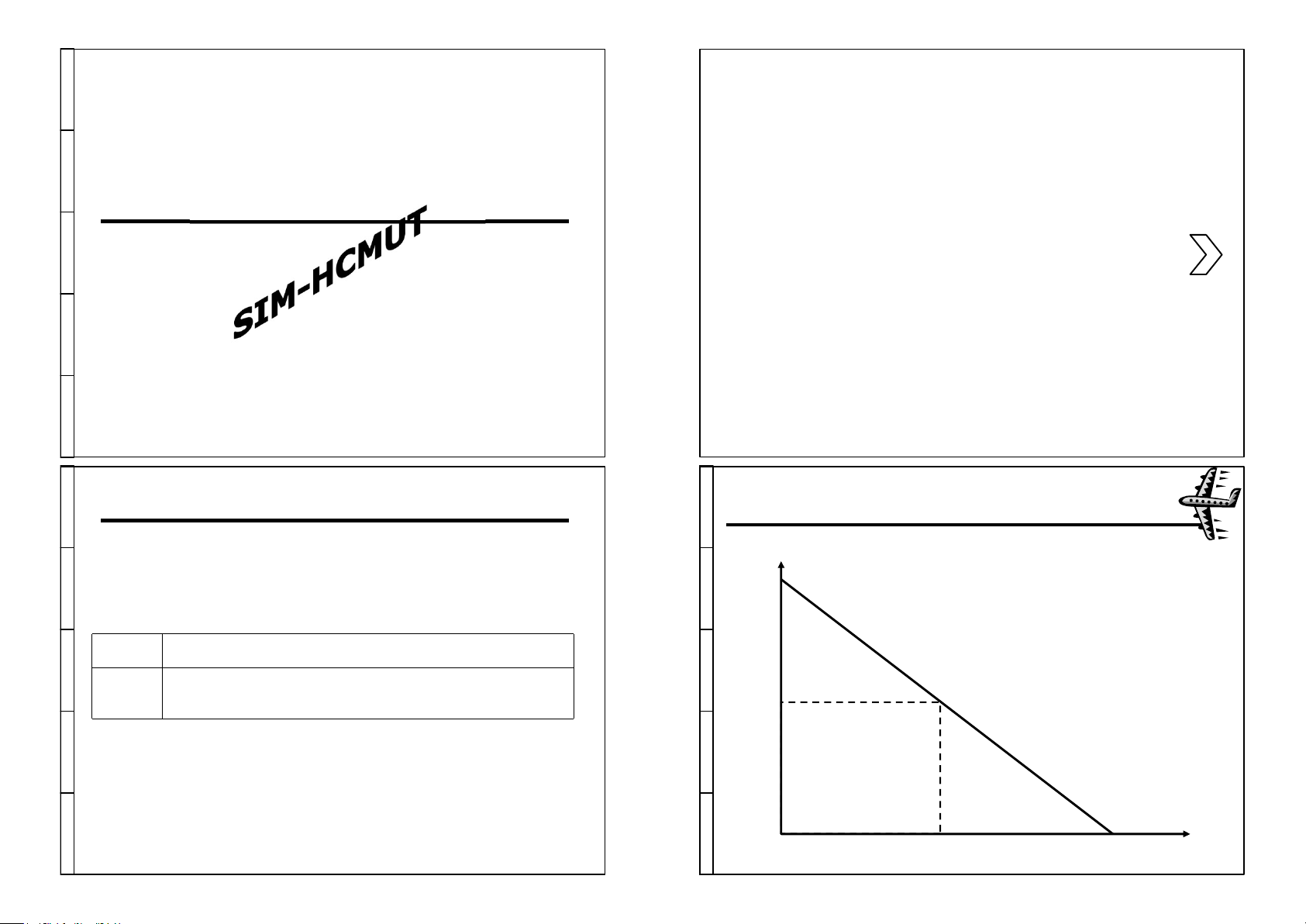
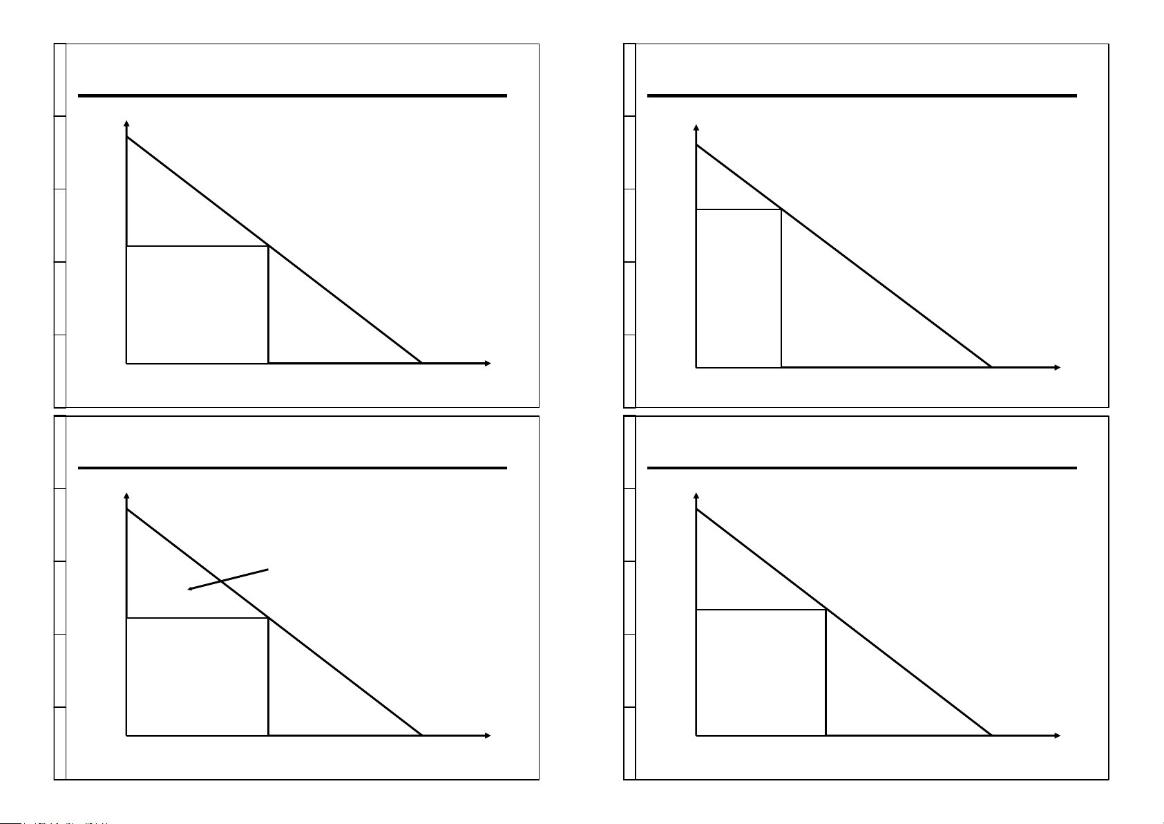
• A ship with C=400 identical cabins 2000
• The Price-Quantity relationship P=2000-2Q 3 Pricing 4
Inventory and warehouse management 1000 2 No. seats Nguyen Thi Duc Nguyen, PhD 4 1 Revenue Management: Example Revenue Management: Example
What is the price that the company Price
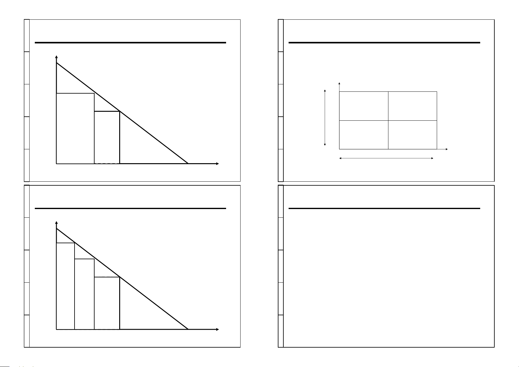
should charge to maximize revenue? Price Revenue=480,000 P2=1600 P0=1200 C=400 No. seats Q2=200 No. seats 5 7 Revenue Management: Example Revenue Management: Example Price Price Money on the Table=160,000 P1=1200 P0=1200 C=400 No. seats C=400 No. 6 seats 8 2 Revenue Management: Example Revenue Management: Example
How can the firm prevent customers from moving from one class to another? Price •
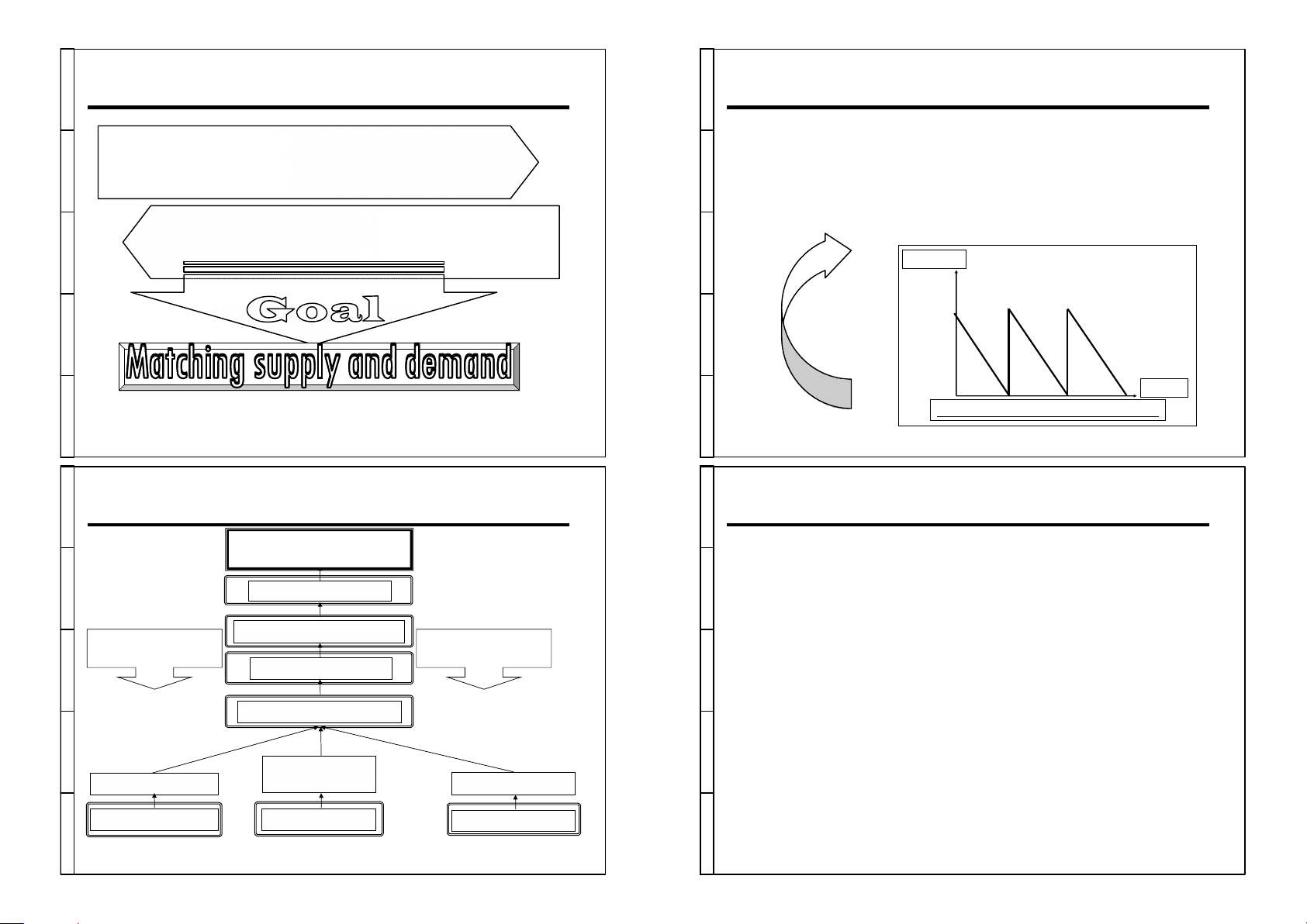
“Allocating the right type of capacity to the right kind of Sensitivity to Duration
customer at the right price so as to maximize revenue or yield”
Revenue=1600(200) + 1200(400-200)=560,000 Sensitivity to Flexibility •
Traditional Industries: Airlines; Hotels; Rental Car Agencies; Retail Industry Low P2=1600 Leisure No P Travelers 1=1200 Demand High No Business Travelers Offer Sensitivity to Price Q High Low 2=200 Q1 =400 No. seats 9 11 Revenue Management: Example Smart Pricing Can we increase revenue more? • Customized Pricing Price
üRevenue Management Techniques
• Distinguish between customers according to their P3=1800 Revenue=1800(100) + 1600(200- price sensitivity 100) + 1200(400-200)=580,000
üInfluence retailer pricing strategies P2=1600
üMove supply chain partners toward global optimization P1=1200 • Dynamic Pricing
üChanging prices over time without necessarily
distinguishing between different customers
üFind the optimal trade-off between high price and low Q2=200 Q
demand versus low price and high demand 1 =400 Q No. 3=100 seats 10 12 3 Smart Pricing Discussion • • Limited Capacity
How does your SC case apply Smart Pricing? When does • Demand Variability Dynamic Pricing Provide Significant
• Seasonality in Demand Pattern Profit Benefit? • Short Planning Horizon A Word of Caution
•Amazon.com experimented with dynamic pricing – customers responded negatively
•Coca-Cola distributors rebel ed against a seasonal pricing scheme 13 1-15 Smart Pricing
The Internet makes Smart Pricing Possible • Low Menu Cost • Low Buyer Search Cost • Visibility
• To the back-end of the supply chain al ows to coordinate pricing, production and distribution 2. Inventory management • Customer Segmentation
• Difficult in conventional stores and easier on the Internet • Testing Capability 14 16 4 RIo N le V E o Nf T In O v R e Y nt M o A r N y A in G Eth M e E S N u T pply Chain Cycle Inventory
Understocking: Demand exceeds amount available
–Lost margin and future sales
Overstocking: Amount available exceeds demand
– Liquidation, Obsolescence, Holding Inventory Q Time t
Cycle inventory = lot size/2 = Q/2 17 1-17 19 INVENTORY S u M p A p N ly A GC Eha M i E n NT
Economics of Scale to Exploit Fixed Costs — Economic Order Quantity— I Im m p prro o v v e e M M a a t t ching g o f o fS u S p u p p ly ply and Demand n Improved Forecasting
» D= Annual demand of the product Reduce Material Flow Time » Cost Availability
S= Fixed cost incurred per order Efficiency Responsiveness Reduce Waiting Time » C= Cost per unit
» h=Holding cost per year as a fraction of product cost Reduce Buffer Inventory
» H=Holding cost per unit per year =hC Supply / Demand » Q=Lot size Economies of Scale Variability Seasonal Variability » n=Order frequency Cycle Inventory Safety Inventory Seasonal Inventory 18 18 20 5
Lot Sizing for a Single Product (EOQ) Example
► Annual order cost =(D/Q)S=ns
5 Demand， D =1,000 units/month = 12,000 units/year
5 Fixed cost, S = $4,000/order; Unit cost, C = $500; Holding cost, h = 20% = 0.2
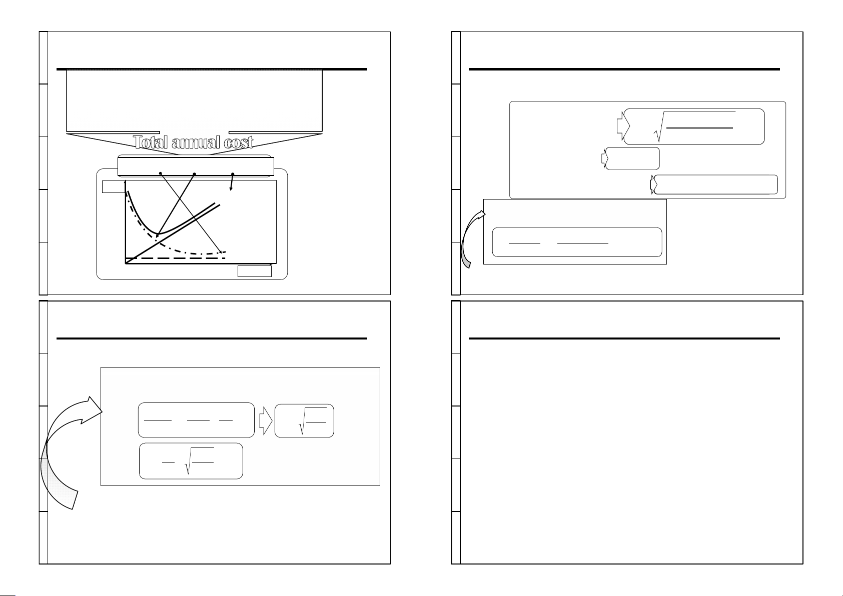
Annual holding cost = (Q/2)H =(Q/2)hC Annual material cost = CD 2X12000X4000 》Optimal order size Q = = 980 0.2X500 》Cycle inventory Q/2 =490 TC =CD + (D/Q)S + (Q/2)hC Cost
》Numbers of orders per year D / Q = 12000 / 980 =12.24 Total Cost Holding Cost
► If we want to reduce the optimal lot size from 980 to 200,
then how much the order cost per lot should be.
> If we increase the lot size by
10% (from 980 to 1100), what the Order Cost hC(Q*)2 S = 0.2X500X2002 = = $166.7 total cost would be. 2D 2X12000 Material Cost
Annual cost = $ 98,636 (from $ Lot Size
97,980)(an increase by only 0.6% (Note: material cost is not 21 included) 23
Lot Sizing for a Single Product
(EOQ ーEconomic Order Quantity)
Aggregating Multiple Products in a Single Order
• One of major fixed costs is transportation
Total annual cost, TC =CD + (D/Q)S + (Q/2)hc
Optimal lot size, Q is obtained by taking the first derivative
► Ways to lower receiving or loading costs: d T ( C) D - S hC = + =0 * D 2 S Q =
》 Aggregating across the products from the same supplier dQ Q2 2 hC
》 Single delivery from multiple suppliers
》 Single delivery to multiple retailers * D DhC n = = * Q S 2 22 24 6