Tiểu luận chủ đề A case study of elegant rugs company môn Business Cost Management | Đại học kinh tế Quốc dân

lOMoAR cPSD| 58511332
TRƯỜNG ĐẠI HỌC KINH TẾ QUỐC DÂN -------***------- ASSIGNMENT
SUBJECT: COST MANAGEMENT
TOPIC: A CASE STUDY OF ELEGANT RUGS COMPANY
Lecturer: PhD. Nguyen Thi Hong Tham
Credit class: QTTH1116E(224)_CLC_01
Group members: Trần Nguyễn Hà My - 11230116
Hoàng Thanh Quang – 11236561
Nguyễn Quỳnh Chi -11231286 Phan Ngọc Linh – 11236423
Nguyễn Công Minh – 11231729 Hà Nội, tháng 3 năm 2025 lOMoAR cPSD| 58511332 TABLE OF CONTENTS
START...........................................................................................................................1
CASE & WORK DIVISION .........................................................................................3
PART A...............................................................................................................5 PART
B...............................................................................................................9
PART C.............................................................................................................11
PART D.............................................................................................................15
PART E&F........................................................................................................18 lOMoAR cPSD| 58511332 [Case]
Consider Elegant Rugs, which uses state-of-the-art automated weaving machines to
produce carpets for homes and offices. Management has altered manufacturing processes
and wants to introduce new styles of carpets. Elegant Rugs’s manager wants to estimate
the indirect manufacturing labor costs per machine-hour of alternative styles of carpets and
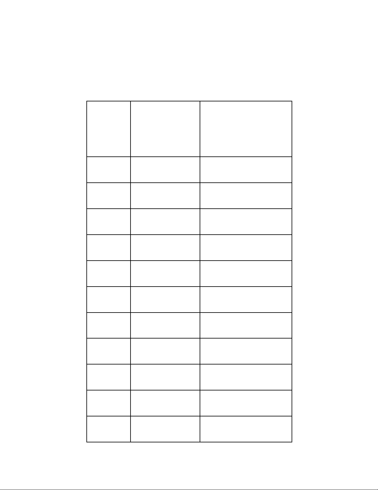
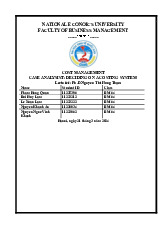
from that choose the most profitable styles to produce. Week Cost Driver: Indirect Manufacturing Machine-Hours Labor Costs (X) (Y) 1 68 $ 1,190 2 88 1,211 3 62 1,004 4 72 917 5 60 770 6 96 1456 7 78 1,180 8 46 710 9 82 1,316 10 94 1,032 11 68 752 lOMoAR cPSD| 58511332 12 48 963 Total 862 $ 12,501 [Required]
a, Apply the six-steps of cost estimation in Elegant Rugs (Step 4: Plot the data) b, Use
the high-low method to compute the indirect manufacturing labor costs c, Suppose
Elegant Rugs’ indirect manufacturing labor costs in week 6 were $1,280, instead of
$1,456, and that 96 machine-hours were used. In this case, the highest observation of
the cost driver (96 machine-hours in week 6) will not coincide with the newer highest
observation of the costs ($1,316 in week9). How would this change affect our high-low
calculation? Given that the cause-and-effect relationship runs from the cost driver to the
costs in a cost function d, Apply the regression analysis methods of cost estimation,
estimate the regressionequation e, Draw the regression line and evaluate it g, Which
methods should Elegant Rugs’s manager use? Why (Explain the implementation issues of the methods) Part Personal in charge A Phan Ngọc Linh B Hoàng Thanh Quang C Nguyễn Công Minh D Nguyễn Quỳnh Chi E,F Trần Nguyễn Hà My
a, Apply the six-steps of cost estimation in Elegant Rugs (Step 4: Plot the data)
– Person in charge: Phan Ngọc Linh
Step 1: Identify the Cost Object
Choose the dependent variable. Which dependent variable (the cost to be predicted and
managed) managers choose will depend on the specific cost function being estimated.
In the Elegant Rugs example, the dependent variable is indirect manufacturing labor costs.
Step 2: Identify the Cost Driver
1. Definition of the Independent Variable (Cost Driver) lOMoAR cPSD| 58511332
- The independent variable is the factor used to predict the dependent variable (costs).
- When the cost is an indirect cost, the independent variable is also called the costallocation base.
- In the Elegant Rugs case, the independent variable must be identified to estimate
indirect manufacturing labor costs.
2. Economic Plausibility
- The cost driver should be measurable and have an economically plausible
relationship with the dependent variable.
- This relationship can be based on physical processes, contractual agreements, or knowledge of operations.
- It must make sense to both the operating manager and the management accountant.
3. Homogeneous Cost Pools
- All cost items in the dependent variable should share the same cost driver.
- If different cost items have different cost drivers, the management accountant
should consider breaking them into separate homogeneous cost pools and
estimating multiple cost functions.
4. Example of Homogeneous Cost Pools -
Fringe Benefits and Cost Drivers:
Health benefits & cafeteria meals → Number of employees.
Pension benefits & life insurance → Employees' salaries.
- Cost items with the same cost driver can be grouped into a single homogeneous
cost pool for more accurate estimation. Application to Elegant Rugs
- In the Elegant Rugs case, machine-hours can be used as the cost driver for indirect
manufacturing labor costs, as there is an economically plausible relationship
between production activity and incurred costs.
- If multiple factors influence indirect labor costs, the company should consider
creating additional cost pools and using more than one independent variable. Step
3: Collect Data on the Cost Object and Cost Driver
1. Importance of Data Collection
- This is one of the most challenging steps in cost analysis.
- Management accountants gather data from company records, interviews with
managers, and special studies. 2. Types of Data - Time-Series Data: lOMoAR cPSD| 58511332
Collected over successive past periods for the same entity (e.g., company, plant, or activity).
Example: Weekly records of Elegant Rugs’ indirect manufacturing
labor costs and machine-hours.
Ideal when operations remain stable without significant economic or technological changes.
Consistent measurement periods are essential.
- Cross-Sectional Data:
Collected from different entities within the same time period.
Example: Comparing personnel costs and loan processing data
across 50 bank branches in a given month.
Effective when entities have a similar relationship between the cost driver and costs.
3. Challenges in Data Collection
- Economic and technological changes can affect data reliability.
- Data inconsistencies may arise if measurement periods vary.
Application to Elegant Rugs •
The company uses time-series data, as it tracks indirect labor costs and
machinehours over multiple weeks. •
Data collection should ensure consistency and account for external factors that
may impact cost relationships. Step 4: Plot the Data
1. Purpose of Plotting the Data
- Helps visualize the relationship between the cost driver and costs.
- Determines whether the relationship is approximately linear. - Identifies the
relevant range of the cost function.
2. Key Insights from the Plot
- If the cost driver and costs exhibit a positive linear relationship, it suggests that
as machine-hours increase, indirect labor costs also increase.
- Helps detect extreme observations (outliers) that may indicate data recording
errors or unusual events (e.g., work stoppages).
3. Application to Elegant Rugs
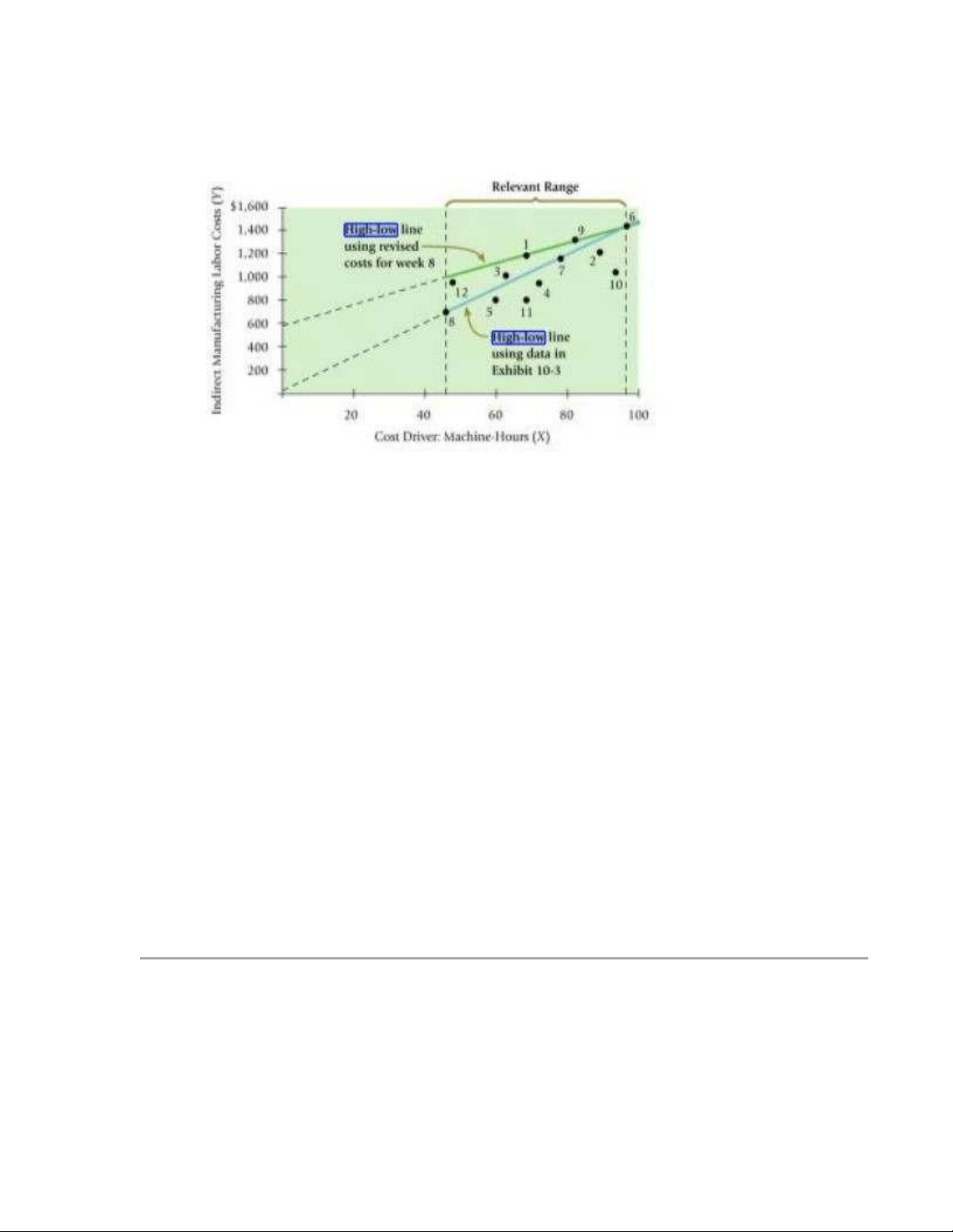
- The plot of machine-hours vs. indirect manufacturing labor costs shows a strong linear relationship. lOMoAR cPSD| 58511332
- The relevant range is 46 to 96 machine-hours per week (from the lowest and highest recorded values).
- No extreme observations were identified, meaning the data is reliable for further analysis.
Step 5: Select and Apply a Cost Estimation Method
1. Purpose of Estimating a Cost Function •
Helps predict costs based on a cost driver. •
Used by managers and accountants to understand cost behavior.
2. Common Methods for Estimation High-Low Method:
o A simple approach to estimating the cost function.
o Uses only the highest and lowest values of the cost driver to determine a linear cost function.
o Provides a basic understanding of cost estimation. Regression Analysis:
o A more advanced and accurate method. o Uses all available data points to
find the best-fitting cost function.
o Often performed using software like Excel.
3. Application to Elegant Rugs
- Managers may use the high-low method to develop an initial cost estimate.
- Regression analysis is preferable for more precise cost estimation.
- The choice of method depends on data availability and the level of accuracy needed.
Step 6: Evaluate the Cost Estimate
- The regression model provides a reasonable fit, but additional statistical analysis
(such as R-squared) would help confirm its accuracy.
- If more precision is needed, a regression approach using least squares would be ideal.
- The cost estimation can now be used for decision-making in selecting the most profitable carpet styles. lOMoAR cPSD| 58511332
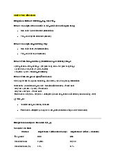
b, Use the high-low method to compute the indirect manufacturing labor costs
Person in charge: Hoang Thanh Quang
- The high-low equation is as follows: Y = a + (b x X)
Y = the value of the estimated cost (Total cost = Fixed cost + Variable cost) a = the
intercept, a fixed quantity for the value of Y when X = 0 ( Fixed cost = Total cost −
Estimated variable cost) b = the slope of the line (unit variable cost)
X = the cost driver, the number of operating hours
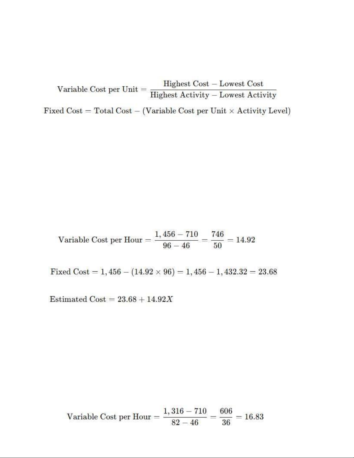
The High-Low method determines variable and fixed costs using two data points:
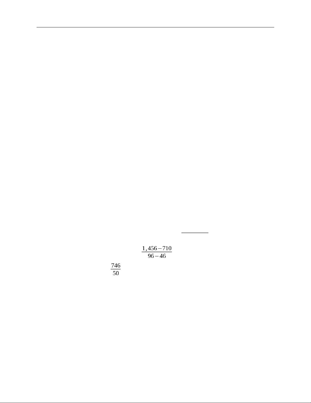
• Highest machine hours (X_max): o Week 6: X = 96, Y = 1,456
• Lowest machine hours (X_min): o Week 8: X = 46, Y = 710
1. Determine the variable cost per machine hour: Y max−Y min Variable = Xmax−Xmin ¿ ¿ =14.92
2. Determine the fixed cost (FC):
Using the total cost equation: Y=FC+(Variable × X )
Substituting values from Week 6:
1,456=FC+(14.92×96)
1,456=FC+1,432.32
FC=1, 456−1,432.32=23.68 3.
Indirect labor cost equation: lOMoAR cPSD| 58511332 Y=23.68+14.92X
This equation can be used to estimate indirect labor costs based on different machine hour values.
- The blue line represents the estimated cost function using the high-low method,
connecting the highest and lowest machine-hour observations.
- The green line represents the high-low cost estimation using revised costs for
week 8. Compared to the blue line, the green line has a slightly different slope and
intercept due to adjustments in the cost values.
- Both lines estimate the relationship between machine-hours (X) and indirect
manufacturing labor costs (Y) within the relevant range (46-96
machinehours). The difference suggests that the revised data for week 8 affected
the cost function, leading to a slightly different approximation of variable and fixed costs.
c, Suppose Elegant Rugs’ indirect manufacturing labor costs in week 6 were $1,280,
instead of $1,456, and that 96 machine-hours were used. In this case, the highest
observation of the cost driver (96 machine-hours in week 6) will not coincide with the
newer highest observation of the costs ($1,316 in week9). How would this change
affect our high-low calculation? Given that the cause-and-effect relationship runs
from the cost driver to the costs in a cost function
Person in charge: Nguyen Cong Minh lOMoAR cPSD| 58511332 1.
The Value and Pitfalls of the High-Low Method
The high-low method is a simple and quick approach to estimating cost behavior. It
allows managers at Elegant Rugs to get an initial understanding of how machine-hours
(cost driver) affect indirect manufacturing labor costs (Y). The formula for cost estimation is:
While this method is useful for quick estimates, it relies only on two data points,
making it sensitive to extreme values or abnormal conditions, which can lead to misleading results. 2.
Initial High-Low Calculation (Before Changes in Week 6 & 8) From the given data:
• Highest Machine-Hours = 96 (Week 6), Cost = $1,456
• Lowest Machine-Hours = 46 (Week 8), Cost = $710 Using the high- low method:
Using Week 6 to find Fixed Cost:
Thus, the estimated cost function is: 3.
Impact of Changing Week 6’s Cost
Now, suppose Week 6’s cost was $1,280 instead of $1,456. •
The highest cost value now shifts to Week 9: $1,316 (82 hours) instead of Week 6. New high-low points: •
High: Week 9 → 82 hours, $1,316 •
Low: Week 8 → 46 hours, $710 New variable cost: lOMoAR cPSD| 58511332
Using Week 9 to find Fixed Cost: New cost function:
Implications of Changing Week 6’s Cost
1. Higher Variable Cost Per Hour ($16.83 vs. $14.92)
- The new estimation suggests a higher marginal cost per machine-hour, which
could impact pricing and profitability decisions.
2. Negative Fixed Cost (-$64.06) is Unrealistic
- A negative fixed cost is not logical, indicating that using Week 9 instead of
Week 6 as the high point skews results.
- The relationship between machine hours and indirect costs may not be purely linear. 4.
Further Change: Adjusting Week 8’s Cost
Now, let’s assume Week 8’s cost was $1,000 instead of $710 due to a labor contract
guaranteeing a minimum payment.
The high-low points remain the same:
o High: Week 9 → 82 hours, $1,316 o
Low: Week 8 → 46 hours, $1,000 New variable cost: New fixed cost: New cost function:
Implications of Changing Week 8’s Cost
1. Much Lower Variable Cost per Machine Hour ($8.78 vs. $14.92 and $16.83)
- This significantly changes cost estimations, making prior pricing decisions potentially incorrect. lOMoAR cPSD| 58511332
- The company might have been overestimating variable costs, leading to overly cautious pricing.
2. Much Higher Fixed Cost ($596.04 vs. $23.68 or -$64.06)
- This suggests fixed costs are more substantial than originally assumed.
- It also highlights how sensitive the high-low method is to one-time adjustments like labor contracts. 5.
Cause-and-Effect Relationship Between Cost Driver and Costs
Given that the cause-and-effect relationship runs from the cost driver (machine-hours) to
the costs in a cost function, changes in cost observations can distort the cost estimation
process. The high-low method assumes that machine-hours are the primary factor driving
costs, but fluctuations due to contractual obligations, seasonal variations, or operational
inefficiencies can introduce errors. In the revised scenario, the cost function changes
significantly when selecting different high and low points, which indicates that external
factors may be influencing labor costs. To improve accuracy, managers should identify
additional cost drivers and analyze historical trends to ensure that the estimated cost
function truly reflects operational reality. 6.
The Danger of Relying on the High-Low Method
As shown in Exhibit 10-5, all other data points lie on or below the estimated cost
function line when Week 8’s cost is changed to $1,000. This demonstrates that the highlow
method can produce misleading results if extreme or non-representative data points are chosen. To mitigate this:
1. Modify the High-Low Method to Use Representative Points
- Instead of blindly using the absolute highest and lowest machine-hours, managers
should pick two observations that best represent normal operations.
- This prevents abnormal events (such as labor contract guarantees) from
distorting cost estimates. 7.
Managerial Recommendations
Given the limitations of the high-low method, Elegant Rugs' management should:
1. Avoid Using the High-Low Method Alone for Cost Estimation
- While useful for quick estimates, it should not be the sole basis for decisionmaking.
- Extreme data points can lead to misleading cost assumptions.
2. Identify and Control Other Cost Drivers
- The assumption that machine-hours are the only cost driver may not hold true. lOMoAR cPSD| 58511332
- Other factors like overtime wages, raw material costs, and machine maintenance should be analyzed.
3. Adjust Pricing Strategies Based on More Accurate Cost Estimations
- If variable costs are lower than previously estimated, carpet prices may need
revision to remain competitive.
- Fixed costs should also be accurately assessed to ensure sustainable pricing. 8. Final Conclusion
The high-low method is a good starting point for estimating cost behavior but is not always reliable. •
Changes in cost data (like those in Week 6 and Week 8) dramatically alter the estimated cost function. •
Managers must modify the method to use representative data points rather
than just picking the highest and lowest machine-hours.
d, Apply the regression analysis methods of cost estimation, estimate the
regression-equation Person in charge: Nguyen Quynh Chi
Linear regression provides a more precise estimate by using all data points instead of just the high-low method.
We perform Ordinary Least Squares (OLS) Regression to estimate the equation: This requires:
- Slope (b): Measures the rate of cost change per machine-hour.
- Intercept (a): Represents fixed costs.
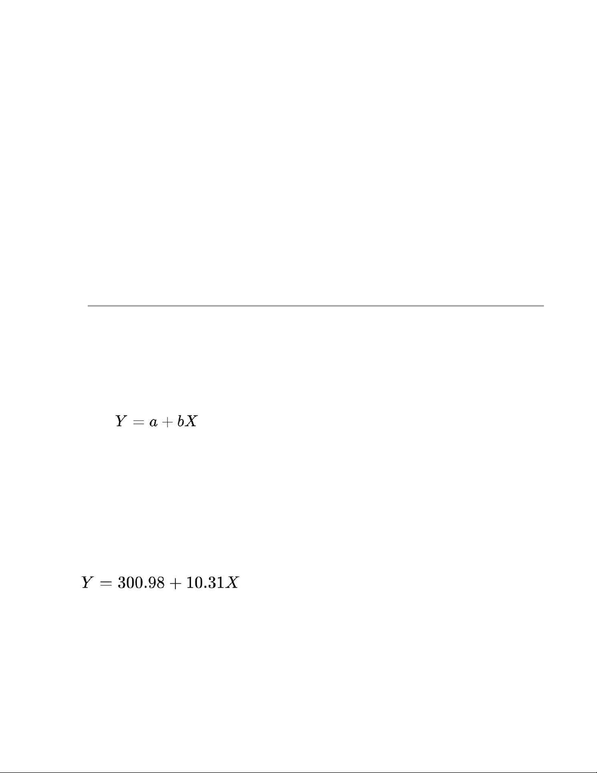
- R² Value: Measures the goodness of fit. 1. Regression Equation
We calculated the linear regression equation as: Where: •
Y: Predicted indirect manufacturing labor cost (in dollars). • X: Number of machine-hours. •
300.98 (Intercept): This represents the fixed labor cost, meaning even if no
machines are running (X = 0), the company still incurs $301 in labor costs. lOMoAR cPSD| 58511332 •
10.31 (Slope): This represents the variable labor cost, meaning that for each
additional machine-hour, the labor cost is expected to increase by $10.31. Example Interpretation: •
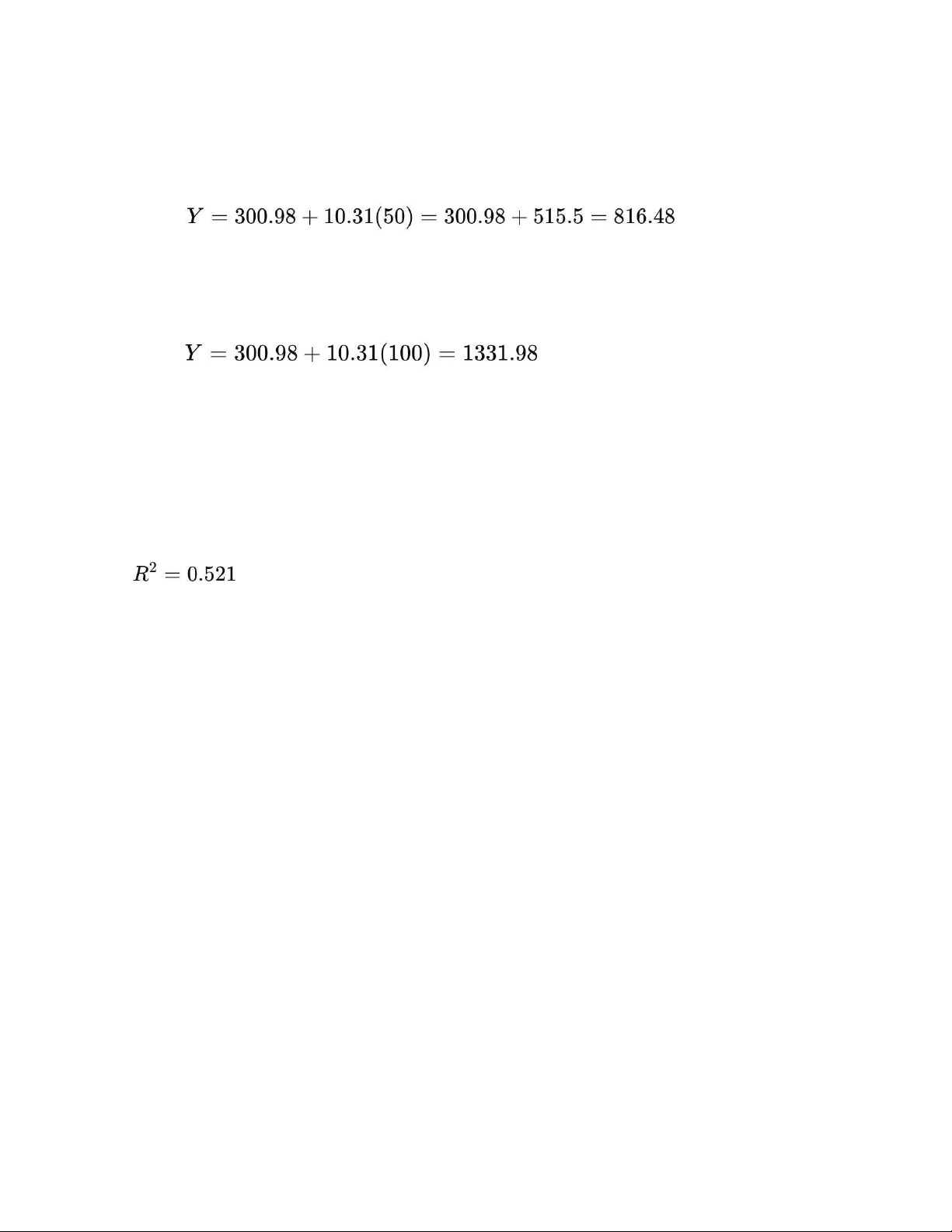
If 50 machine-hours are used, the predicted labor cost is:
So, for 50 machine-hours, the estimated labor cost is $816.48. •
If 100 machine-hours are used, the predicted labor cost is:
So, for 100 machine-hours, the estimated labor cost is $1331.98.
This equation helps forecast labor costs based on machine-hours.
2. Model Performance: How Well Does It Fit the Data?
We use R-squared (R2R^2) to measure how well machine-hours explain the variation in labor costs. •
The model explains 52.1% of the variation in labor costs. •
The remaining 47.9% is due to other factors not included in the model. •
This is a moderate fit: machine-hours impact labor costs, but other variables also contribute.
3. Limitations and How to Improve the Model
Since R^2 = 0.521 is not very high, it indicates that machine-hours alone are not the only
factor driving labor costs. Possible reasons and improvements:
A. Other Factors Affecting Labor Costs
1. Overtime and Labor Efficiency: If workers work overtime, labor costs could be higher than predicted.
2. Material Handling and Setup Costs: Some carpet styles might require more labor,
even with the same machine-hours.
3. Different Wage Rates: If different workers operate the machines, wage
differencesmight impact labor costs.
4. Breakdowns and Idle Time: If machines break down, laborers may still be paid
even though production is stopped.
Solution: Include more variables in the model, such as: lOMoAR cPSD| 58511332 • Overtime hours • Number of workers per shift • Carpet type produced • Breakdown time B. Non-Linear Relationships •
The relationship between machine-hours and labor costs might not be perfectly linear. •
If increasing machine-hours leads to higher efficiency, then labor costs might
increase at a decreasing rate.
Solution: Try non-linear regression (e.g., quadratic models) to see if it better fits the data.
4. Practical Use of This Regression Model
A. Cost Estimation & Forecasting •
The manager at Elegant Rugs can use this model to estimate future labor costs. •
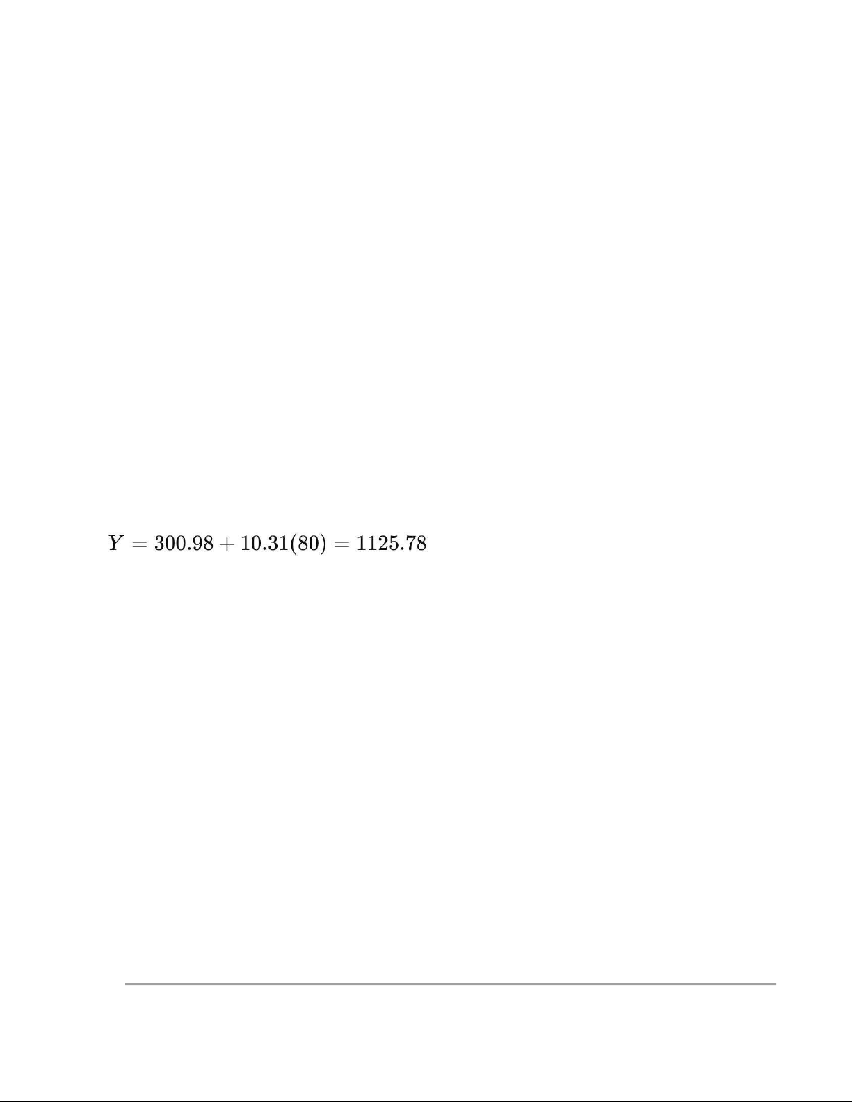
Example: If the company plans to run 80 machine-hours next week, the estimated labor cost is:
This helps in budgeting and financial planning.
B. Decision-Making on Machine Usage •
If labor costs increase faster than expected, the company might need to optimize machine scheduling. •
Example: If machine-hours increase by 10, the additional labor cost is $103.10. •
If that cost is too high, the company may need to find ways to improve efficiency.
C. Identifying Cost-Saving Strategies
1. Reducing Idle Time: If machines are not running efficiently, reducing downtime can lower labor costs.
2. Training Workers: Better-trained workers may handle the machines more efficiently, reducing costs.
3. Optimizing Work Shifts: Adjusting shift schedules could help reduce overtime costs. lOMoAR cPSD| 58511332
e, Draw the regression line and evaluate it Person
in charge: Tran Nguyen Ha My
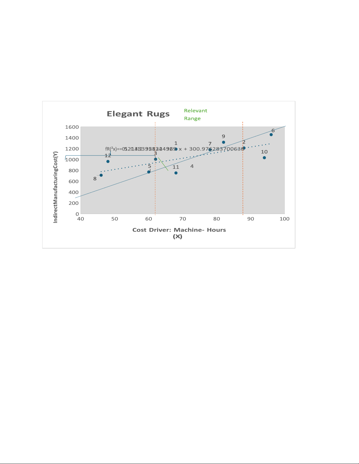
Excel estimates the cost function to be y = $300.98 + $10.31X
The regression line is derived using the least-squares technique. The least-squares
technique determines the regression line by minimizing the sum of the squared vertical
differences from the data points (the various points in the graph) to the regression line. The
vertical difference, called the residual term, measures the distance between actual cost and
estimated cost for each observation of the cost driver. The smaller the residual terms, the
better is the fit between the actual cost observations and estimated costs. Goodness of
fit indicates the strength of the relationship between the cost driver and costs. The
regression line rises from left to right. The positive slope of this line and small residual
terms indicate that, on average, indirect manufacturing labor costs increase as the number of machine-hours increases. lOMoAR cPSD| 58511332 Calculate R², intercept, t-value- pvalue,.. using LINEST function on Excel LINEST(known_y' s, [known_x's],
[const], [stats]) Statist Functions ics R² =RSQ(B3: B14;A3:A 14) INTE =INTERC RCEP EPT(B3:B T 14, A3:A14) Slope =SLOPE( B2:B6, A2:A6) Standa =STEYX( rd Error B2:B6, (SE) A2:A6) t-value =SLOPE( B2:B6, A2:A6)/ST EYX(B2:B 6, A2:A6) pvalue =T.DIST.2 T(ABS(t- value), df) lOMoAR cPSD| 58511332
Here is a picture of my results using the above functions to calculate the indexes on
Excel, I also drew Regression Line on Excel
R² = 0.5214 means that 52.14% of the variance in the dependent variable (Y) is
explained by the independent variable (X)
SE = 170.54 is large compared to the slope (10.31), meaning the estimates are uncertain.
g, Which methods should Elegant Rugs’s manager use? Why (Explain the
implementation issues of the methods)
Elegant Rugs should use the regression method. The regression method is more accurate
than the high-low method because the regression equation estimates costs using
information from all observations, whereas the high-low equation uses information from
only two observations. The inaccuracies of the high-low method can mislead managers.
For instance, if 90 machine-hours are budgeted for the upcoming week, we could have a small compare on this table: The high-low method equation
The regression analysis equation lOMoAR cPSD| 58511332
In the preceding section:
y = $23.68 + ($14.92 per machine-hour X y = $300.98 + ($10.31 per machine-hour Number of machine-hours). X 90 machine-hours)
For 90 machine-hours, the predicted For 90 machine-hours, the predicted weekly costs are weekly costs are
$23.68 + ($14.92 per machine-hour X 90 $23.68 + ($14.92 per machine-hour X 90
machine-hours) = $1,366.48
machine-hours) = = $1,228.88
Suppose that for 7 weeks over the next 12-week period, Elegant Rugs runs its machines for
90 hours each week. Assume the average indirect manufacturing labor costs for those 7 weeks are $1,300.
$1,228.88 < $1,300 < $1,300
Based on the high-low method prediction of $1,366.48, Elegant Rugs would conclude it
has performed well because actual costs are less than predicted costs. But comparing the
$1,300 performance with the more-accurate $1,228.88 prediction of the regression model
tells a different story and would probably prompt Elegant Rugs to search for ways to improve its cost performance.