Time Series Analysis and Its Application with R examples | Sách Tiếng Anh
Time Series Analysis and Its Application with R examples | Sách Tiếng Anh . Tài liệu giúp bạn tham khảo, ôn tập và đạt kết quả cao. Mời đọc đón xem!
Môn: Tiếng Anh chuyên ngành 363 tài liệu
Trường: Tài liệu Tiếng Anh chuyên ngành, Tiếng Anh cho người đi làm 466 tài liệu
Tác giả:


Preview text:
Springer Texts in Statistics Series Editors G. Casella S. Fienberg I. Olkin
For other titles published in this series, go to www.springer.com/series/417
Robert H. Shumway • David S. Stoffer Time Series Analysis and Its Applications With R Examples Third edition Prof. Robert H. Shumway Prof. David S. Stoffer Department of Statistics Department of Statistics University of California University of Pittsburgh Davis, California Pittsburgh, Pennsylvania USA USA ISSN 1431-875X ISBN 978-1-4419-7864-6 e-ISBN 978-1-4419-7865-3 DOI 10.1007/978-1-4419-7865-3
Springer New York Dordrecht Heidelberg London
© Springer Science+Business Media, LLC 2011
All rights reserved. This work may not be translated or copied in whole or in part without the written
permission of the publisher (Springer Science+Business Media, LLC, 233 Spring Street, New York,
NY 10013, USA), except for brief excerpts in connection with reviews or scholarly analysis. Use in
connection with any form of information storage and retrieval, electronic adaptation, computer
software, or by similar or dissimilar methodology now known or hereafter developed is forbidden.
The use in this publication of trade names, trademarks, service marks, and similar terms, even if they
are not identified as such, is not to be taken as an expression of opinion as to whether or not they are
subject to proprietary rights. Printed on acid-free paper
Springer is part of Springer Science+Business Media (www.springer.com)
To my wife, Ruth, for her support and joie de vivre, and to the
memory of my thesis adviser, Solomon Kullback. R.H.S.
To my family and friends, who constantly remind me what is important. D.S.S. Preface to the Third Edition
The goals of this book are to develop an appreciation for the richness and
versatility of modern time series analysis as a tool for analyzing data, and still
maintain a commitment to theoretical integrity, as exemplified by the seminal
works of Brillinger (1975) and Hannan (1970) and the texts by Brockwell and
Davis (1991) and Fuller (1995). The advent of inexpensive powerful computing
has provided both real data and new software that can take one considerably
beyond the fitting of simple time domain models, such as have been elegantly
described in the landmark work of Box and Jenkins (1970). This book is
designed to be useful as a text for courses in time series on several different
levels and as a reference work for practitioners facing the analysis of time-
correlated data in the physical, biological, and social sciences.
We have used earlier versions of the text at both the undergraduate and
graduate levels over the past decade. Our experience is that an undergraduate
course can be accessible to students with a background in regression analysis
and may include §1.1–§1.6, §2.1–§2.3, the results and numerical parts of §3.1–
§3.9, and briefly the results and numerical parts of §4.1–§4.6. At the advanced
undergraduate or master’s level, where the students have some mathematical
statistics background, more detailed coverage of the same sections, with the
inclusion of §2.4 and extra topics from Chapter 5 or Chapter 6 can be used as
a one-semester course. Often, the extra topics are chosen by the students ac-
cording to their interests. Finally, a two-semester upper-level graduate course
for mathematics, statistics, and engineering graduate students can be crafted
by adding selected theoretical appendices. For the upper-level graduate course,
we should mention that we are striving for a broader but less rigorous level
of coverage than that which is attained by Brockwell and Davis (1991), the classic entry at this level.
The major difference between this third edition of the text and the second
edition is that we provide R code for almost all of the numerical examples. In
addition, we provide an R supplement for the text that contains the data and
scripts in a compressed file called tsa3.rda; the supplement is available on the
website for the third edition, http://www.stat.pitt.edu/stoffer/tsa3/, viii Preface to the Third Edition
or one of its mirrors. On the website, we also provide the code used in each
example so that the reader may simply copy-and-paste code directly into R.
Specific details are given in Appendix R and on the website for the text.
Appendix R is new to this edition, and it includes a small R tutorial as well
as providing a reference for the data sets and scripts included in tsa3.rda. So
there is no misunderstanding, we emphasize the fact that this text is about
time series analysis, not about R. R code is provided simply to enhance the
exposition by making the numerical examples reproducible.
We have tried, where possible, to keep the problem sets in order so that an
instructor may have an easy time moving from the second edition to the third
edition. However, some of the old problems have been revised and there are
some new problems. Also, some of the data sets have been updated. We added
one section in Chapter 5 on unit roots and enhanced some of the presenta-
tions throughout the text. The exposition on state-space modeling, ARMAX
models, and (multivariate) regression with autocorrelated errors in Chapter 6
have been expanded. In this edition, we use standard R functions as much as
possible, but we use our own scripts (included in tsa3.rda) when we feel it
is necessary to avoid problems with a particular R function; these problems
are discussed in detail on the website for the text under R Issues.
We thank John Kimmel, Executive Editor, Springer Statistics, for his guid-
ance in the preparation and production of this edition of the text. We are
grateful to Don Percival, University of Washington, for numerous suggestions
that led to substantial improvement to the presentation in the second edition,
and consequently in this edition. We thank Doug Wiens, University of Alberta,
for help with some of the R code in Chapters 4 and 7, and for his many sug-
gestions for improvement of the exposition. We are grateful for the continued
help and advice of Pierre Duchesne, University of Montreal, and Alexander
Aue, University of California, Davis. We also thank the many students and
other readers who took the time to mention typographical errors and other
corrections to the first and second editions. Finally, work on the this edition
was supported by the National Science Foundation while one of us (D.S.S.)
was working at the Foundation under the Intergovernmental Personnel Act. Davis, CA Robert H. Shumway Pittsburgh, PA David S. Stoffer September 2010 Contents
Preface to the Third Edition . . . . . . . . . . . . . . . . . . . . . . . . . . . . . . . . . . . vii 1
Characteristics of Time Series . . . . . . . . . . . . . . . . . . . . . . . . . . . . . 1 1.1
Introduction . . . . . . . . . . . . . . . . . . . . . . . . . . . . . . . . . . . . . . . . . . . . 1 1.2
The Nature of Time Series Data . . . . . . . . . . . . . . . . . . . . . . . . . . . 3 1.3
Time Series Statistical Models . . . . . . . . . . . . . . . . . . . . . . . . . . . . 11 1.4
Measures of Dependence: Autocorrelation and
Cross-Correlation . . . . . . . . . . . . . . . . . . . . . . . . . . . . . . . . . . . . . . . . 17 1.5
Stationary Time Series . . . . . . . . . . . . . . . . . . . . . . . . . . . . . . . . . . . 22 1.6
Estimation of Correlation . . . . . . . . . . . . . . . . . . . . . . . . . . . . . . . . . 28 1.7
Vector-Valued and Multidimensional Series . . . . . . . . . . . . . . . . . 33
Problems . . . . . . . . . . . . . . . . . . . . . . . . . . . . . . . . . . . . . . . . . . . . . . . . . . . 39 2
Time Series Regression and Exploratory Data Analysis . . . . 47 2.1
Introduction . . . . . . . . . . . . . . . . . . . . . . . . . . . . . . . . . . . . . . . . . . . . 47 2.2
Classical Regression in the Time Series Context . . . . . . . . . . . . . 48 2.3
Exploratory Data Analysis . . . . . . . . . . . . . . . . . . . . . . . . . . . . . . . . 57 2.4
Smoothing in the Time Series Context . . . . . . . . . . . . . . . . . . . . . 70
Problems . . . . . . . . . . . . . . . . . . . . . . . . . . . . . . . . . . . . . . . . . . . . . . . . . . . 78 3
ARIMA Models . . . . . . . . . . . . . . . . . . . . . . . . . . . . . . . . . . . . . . . . . . . 83 3.1
Introduction . . . . . . . . . . . . . . . . . . . . . . . . . . . . . . . . . . . . . . . . . . . 83 3.2
Autoregressive Moving Average Models . . . . . . . . . . . . . . . . . . . . 84 3.3
Difference Equations . . . . . . . . . . . . . . . . . . . . . . . . . . . . . . . . . . . . . 97 3.4
Autocorrelation and Partial Autocorrelation . . . . . . . . . . . . . . . . 102 3.5 Forecasting
. . . . . . . . . . . . . . . . . . . . . . . . . . . . . . . . . . . . . . . . . . . . 108 3.6
Estimation . . . . . . . . . . . . . . . . . . . . . . . . . . . . . . . . . . . . . . . . . . . . . 121 3.7
Integrated Models for Nonstationary Data . . . . . . . . . . . . . . . . . 141 3.8
Building ARIMA Models . . . . . . . . . . . . . . . . . . . . . . . . . . . . . . . . 144 3.9
Multiplicative Seasonal ARIMA Models . . . . . . . . . . . . . . . . . . . . 154
Problems . . . . . . . . . . . . . . . . . . . . . . . . . . . . . . . . . . . . . . . . . . . . . . . . . . . 162 x Contents 4
Spectral Analysis and Filtering . . . . . . . . . . . . . . . . . . . . . . . . . . . . 173 4.1
Introduction . . . . . . . . . . . . . . . . . . . . . . . . . . . . . . . . . . . . . . . . . . . . 173 4.2
Cyclical Behavior and Periodicity . . . . . . . . . . . . . . . . . . . . . . . . . . 175 4.3
The Spectral Density . . . . . . . . . . . . . . . . . . . . . . . . . . . . . . . . . . . . 180 4.4
Periodogram and Discrete Fourier Transform . . . . . . . . . . . . . . . 187 4.5
Nonparametric Spectral Estimation . . . . . . . . . . . . . . . . . . . . . . . . 196 4.6
Parametric Spectral Estimation . . . . . . . . . . . . . . . . . . . . . . . . . . . 212 4.7
Multiple Series and Cross-Spectra . . . . . . . . . . . . . . . . . . . . . . . . . 216 4.8
Linear Filters . . . . . . . . . . . . . . . . . . . . . . . . . . . . . . . . . . . . . . . . . . . 221 4.9
Dynamic Fourier Analysis and Wavelets . . . . . . . . . . . . . . . . . . . . 228
4.10 Lagged Regression Models . . . . . . . . . . . . . . . . . . . . . . . . . . . . . . . . 242
4.11 Signal Extraction and Optimum Filtering . . . . . . . . . . . . . . . . . . . 247
4.12 Spectral Analysis of Multidimensional Series . . . . . . . . . . . . . . . . 252
Problems . . . . . . . . . . . . . . . . . . . . . . . . . . . . . . . . . . . . . . . . . . . . . . . . . . . 255 5
Additional Time Domain Topics . . . . . . . . . . . . . . . . . . . . . . . . . . . 267 5.1
Introduction . . . . . . . . . . . . . . . . . . . . . . . . . . . . . . . . . . . . . . . . . . . . 267 5.2
Long Memory ARMA and Fractional Differencing . . . . . . . . . . . 267 5.3
Unit Root Testing . . . . . . . . . . . . . . . . . . . . . . . . . . . . . . . . . . . . . . . 277 5.4
GARCH Models . . . . . . . . . . . . . . . . . . . . . . . . . . . . . . . . . . . . . . . . 280 5.5
Threshold Models . . . . . . . . . . . . . . . . . . . . . . . . . . . . . . . . . . . . . . . 289 5.6
Regression with Autocorrelated Errors . . . . . . . . . . . . . . . . . . . . . 293 5.7
Lagged Regression: Transfer Function Modeling . . . . . . . . . . . . . 296 5.8
Multivariate ARMAX Models . . . . . . . . . . . . . . . . . . . . . . . . . . . . . 301
Problems . . . . . . . . . . . . . . . . . . . . . . . . . . . . . . . . . . . . . . . . . . . . . . . . . . . 315 6
State-Space Models . . . . . . . . . . . . . . . . . . . . . . . . . . . . . . . . . . . . . . . . 319 6.1
Introduction . . . . . . . . . . . . . . . . . . . . . . . . . . . . . . . . . . . . . . . . . . . 319 6.2
Filtering, Smoothing, and Forecasting . . . . . . . . . . . . . . . . . . . . . 325 6.3 Maximum Likelihood Estimation
. . . . . . . . . . . . . . . . . . . . . . . . . 335 6.4
Missing Data Modifications . . . . . . . . . . . . . . . . . . . . . . . . . . . . . . 344 6.5
Structural Models: Signal Extraction and Forecasting . . . . . . . . 350 6.6
State-Space Models with Correlated Errors . . . . . . . . . . . . . . . . . 354 6.6.1
ARMAX Models . . . . . . . . . . . . . . . . . . . . . . . . . . . . . . . . . . 355 6.6.2
Multivariate Regression with Autocorrelated Errors . . . . 356 6.7
Bootstrapping State-Space Models . . . . . . . . . . . . . . . . . . . . . . . . 359 6.8
Dynamic Linear Models with Switching . . . . . . . . . . . . . . . . . . . . 365 6.9
Stochastic Volatility . . . . . . . . . . . . . . . . . . . . . . . . . . . . . . . . . . . . . 378
6.10 Nonlinear and Non-normal State-Space Models Using Monte
Carlo Methods . . . . . . . . . . . . . . . . . . . . . . . . . . . . . . . . . . . . . . . . . 387
Problems . . . . . . . . . . . . . . . . . . . . . . . . . . . . . . . . . . . . . . . . . . . . . . . . . . . 398 Contents xi 7
Statistical Methods in the Frequency Domain . . . . . . . . . . . . . 405 7.1
Introduction . . . . . . . . . . . . . . . . . . . . . . . . . . . . . . . . . . . . . . . . . . . . 405 7.2
Spectral Matrices and Likelihood Functions . . . . . . . . . . . . . . . . . 409 7.3
Regression for Jointly Stationary Series . . . . . . . . . . . . . . . . . . . . 410 7.4
Regression with Deterministic Inputs . . . . . . . . . . . . . . . . . . . . . . 420 7.5
Random Coefficient Regression . . . . . . . . . . . . . . . . . . . . . . . . . . . 429 7.6
Analysis of Designed Experiments . . . . . . . . . . . . . . . . . . . . . . . . . 434 7.7
Discrimination and Cluster Analysis . . . . . . . . . . . . . . . . . . . . . . . 450 7.8
Principal Components and Factor Analysis . . . . . . . . . . . . . . . . . 468 7.9 The Spectral Envelope
. . . . . . . . . . . . . . . . . . . . . . . . . . . . . . . . . . 485
Problems . . . . . . . . . . . . . . . . . . . . . . . . . . . . . . . . . . . . . . . . . . . . . . . . . . . 501
Appendix A: Large Sample Theory . . . . . . . . . . . . . . . . . . . . . . . . . . . . 507
A.1 Convergence Modes . . . . . . . . . . . . . . . . . . . . . . . . . . . . . . . . . . . . . . 507
A.2 Central Limit Theorems . . . . . . . . . . . . . . . . . . . . . . . . . . . . . . . . . . 515
A.3 The Mean and Autocorrelation Functions . . . . . . . . . . . . . . . . . . . 518
Appendix B: Time Domain Theory . . . . . . . . . . . . . . . . . . . . . . . . . . . . 527
B.1 Hilbert Spaces and the Projection Theorem . . . . . . . . . . . . . . . . . 527
B.2 Causal Conditions for ARMA Models . . . . . . . . . . . . . . . . . . . . . . 531
B.3 Large Sample Distribution of the AR(p) Conditional Least
Squares Estimators . . . . . . . . . . . . . . . . . . . . . . . . . . . . . . . . . . . . . . 533
B.4 The Wold Decomposition . . . . . . . . . . . . . . . . . . . . . . . . . . . . . . . . . 537
Appendix C: Spectral Domain Theory . . . . . . . . . . . . . . . . . . . . . . . . . 539
C.1 Spectral Representation Theorem . . . . . . . . . . . . . . . . . . . . . . . . . . 539
C.2 Large Sample Distribution of the DFT and Smoothed
Periodogram . . . . . . . . . . . . . . . . . . . . . . . . . . . . . . . . . . . . . . . . . . . . 543
C.3 The Complex Multivariate Normal Distribution . . . . . . . . . . . . . 554
Appendix R: R Supplement . . . . . . . . . . . . . . . . . . . . . . . . . . . . . . . . . . . 559
R.1 First Things First . . . . . . . . . . . . . . . . . . . . . . . . . . . . . . . . . . . . . . . 559
R.1.1 Included Data Sets . . . . . . . . . . . . . . . . . . . . . . . . . . . . . . . . 560
R.1.2 Included Scripts . . . . . . . . . . . . . . . . . . . . . . . . . . . . . . . . . . . 562
R.2 Getting Started . . . . . . . . . . . . . . . . . . . . . . . . . . . . . . . . . . . . . . . . . 567
R.3 Time Series Primer . . . . . . . . . . . . . . . . . . . . . . . . . . . . . . . . . . . . . . 571
References . . . . . . . . . . . . . . . . . . . . . . . . . . . . . . . . . . . . . . . . . . . . . . . . . . . . . 577
Index . . . . . . . . . . . . . . . . . . . . . . . . . . . . . . . . . . . . . . . . . . . . . . . . . . . . . . . . . . 591 1 Characteristics of Time Series 1.1 Introduction
The analysis of experimental data that have been observed at different points
in time leads to new and unique problems in statistical modeling and infer-
ence. The obvious correlation introduced by the sampling of adjacent points
in time can severely restrict the applicability of the many conventional statis-
tical methods traditionally dependent on the assumption that these adjacent
observations are independent and identically distributed. The systematic ap-
proach by which one goes about answering the mathematical and statistical
questions posed by these time correlations is commonly referred to as time series analysis.
The impact of time series analysis on scientific applications can be par-
tially documented by producing an abbreviated listing of the diverse fields
in which important time series problems may arise. For example, many fa-
miliar time series occur in the field of economics, where we are continually
exposed to daily stock market quotations or monthly unemployment figures.
Social scientists follow population series, such as birthrates or school enroll-
ments. An epidemiologist might be interested in the number of influenza cases
observed over some time period. In medicine, blood pressure measurements
traced over time could be useful for evaluating drugs used in treating hy-
pertension. Functional magnetic resonance imaging of brain-wave time series
patterns might be used to study how the brain reacts to certain stimuli under
various experimental conditions.
Many of the most intensive and sophisticated applications of time series
methods have been to problems in the physical and environmental sciences.
This fact accounts for the basic engineering flavor permeating the language of
time series analysis. One of the earliest recorded series is the monthly sunspot
numbers studied by Schuster (1906). More modern investigations may cen-
ter on whether a warming is present in global temperature measurements
R.H. Shumway and D.S. Stoffer, Time Series Analysis and Its Applications: With R Examples, 1
Springer Texts in Statistics, DOI 10.1007/978-1-4419-7865-3_1,
© Springer Science+Business Media, LLC 2011 2
1 Characteristics of Time Series
or whether levels of pollution may influence daily mortality in Los Angeles.
The modeling of speech series is an important problem related to the efficient
transmission of voice recordings. Common features in a time series character-
istic known as the power spectrum are used to help computers recognize and
translate speech. Geophysical time series such as those produced by yearly de-
positions of various kinds can provide long-range proxies for temperature and
rainfall. Seismic recordings can aid in mapping fault lines or in distinguishing
between earthquakes and nuclear explosions.
The above series are only examples of experimental databases that can
be used to illustrate the process by which classical statistical methodology
can be applied in the correlated time series framework. In our view, the first
step in any time series investigation always involves careful scrutiny of the
recorded data plotted over time. This scrutiny often suggests the method of
analysis as well as statistics that will be of use in summarizing the information
in the data. Before looking more closely at the particular statistical methods,
it is appropriate to mention that two separate, but not necessarily mutually
exclusive, approaches to time series analysis exist, commonly identified as the
time domain approach and the frequency domain approach.
The time domain approach is generally motivated by the presumption
that correlation between adjacent points in time is best explained in terms
of a dependence of the current value on past values. The time domain ap-
proach focuses on modeling some future value of a time series as a parametric
function of the current and past values. In this scenario, we begin with linear
regressions of the present value of a time series on its own past values and
on the past values of other series. This modeling leads one to use the results
of the time domain approach as a forecasting tool and is particularly popular
with economists for this reason.
One approach, advocated in the landmark work of Box and Jenkins (1970;
see also Box et al., 1994), develops a systematic class of models called au-
toregressive integrated moving average (ARIMA) models to handle time-
correlated modeling and forecasting. The approach includes a provision for
treating more than one input series through multivariate ARIMA or through
transfer function modeling. The defining feature of these models is that they
are multiplicative models, meaning that the observed data are assumed to
result from products of factors involving differential or difference equation
operators responding to a white noise input.
A more recent approach to the same problem uses additive models more
familiar to statisticians. In this approach, the observed data are assumed to
result from sums of series, each with a specified time series structure; for exam-
ple, in economics, assume a series is generated as the sum of trend, a seasonal
effect, and error. The state-space model that results is then treated by making
judicious use of the celebrated Kalman filters and smoothers, developed origi-
nally for estimation and control in space applications. Two relatively complete
presentations from this point of view are in Harvey (1991) and Kitagawa and
Gersch (1996). Time series regression is introduced in Chapter 2, and ARIMA
1.2 The Nature of Time Series Data 3
and related time domain models are studied in Chapter 3, with the empha-
sis on classical, statistical, univariate linear regression. Special topics on time
domain analysis are covered in Chapter 5; these topics include modern treat-
ments of, for example, time series with long memory and GARCH models
for the analysis of volatility. The state-space model, Kalman filtering and
smoothing, and related topics are developed in Chapter 6.
Conversely, the frequency domain approach assumes the primary charac-
teristics of interest in time series analyses relate to periodic or systematic
sinusoidal variations found naturally in most data. These periodic variations
are often caused by biological, physical, or environmental phenomena of inter-
est. A series of periodic shocks may influence certain areas of the brain; wind
may affect vibrations on an airplane wing; sea surface temperatures caused by El Ni˜
no oscillations may affect the number of fish in the ocean. The study
of periodicity extends to economics and social sciences, where one may be
interested in yearly periodicities in such series as monthly unemployment or monthly birth rates.
In spectral analysis, the partition of the various kinds of periodic variation
in a time series is accomplished by evaluating separately the variance associ-
ated with each periodicity of interest. This variance profile over frequency is
called the power spectrum. In our view, no schism divides time domain and
frequency domain methodology, although cliques are often formed that advo-
cate primarily one or the other of the approaches to analyzing data. In many
cases, the two approaches may produce similar answers for long series, but
the comparative performance over short samples is better done in the time
domain. In some cases, the frequency domain formulation simply provides a
convenient means for carrying out what is conceptually a time domain calcu-
lation. Hopefully, this book will demonstrate that the best path to analyzing
many data sets is to use the two approaches in a complementary fashion. Ex-
positions emphasizing primarily the frequency domain approach can be found
in Bloomfield (1976, 2000), Priestley (1981), or Jenkins and Watts (1968).
On a more advanced level, Hannan (1970), Brillinger (1981, 2001), Brockwell
and Davis (1991), and Fuller (1996) are available as theoretical sources. Our
coverage of the frequency domain is given in Chapters 4 and 7.
The objective of this book is to provide a unified and reasonably complete
exposition of statistical methods used in time series analysis, giving serious
consideration to both the time and frequency domain approaches. Because a
myriad of possible methods for analyzing any particular experimental series
can exist, we have integrated real data from a number of subject fields into
the exposition and have suggested methods for analyzing these data.
1.2 The Nature of Time Series Data
Some of the problems and questions of interest to the prospective time se-
ries analyst can best be exposed by considering real experimental data taken 4
1 Characteristics of Time Series
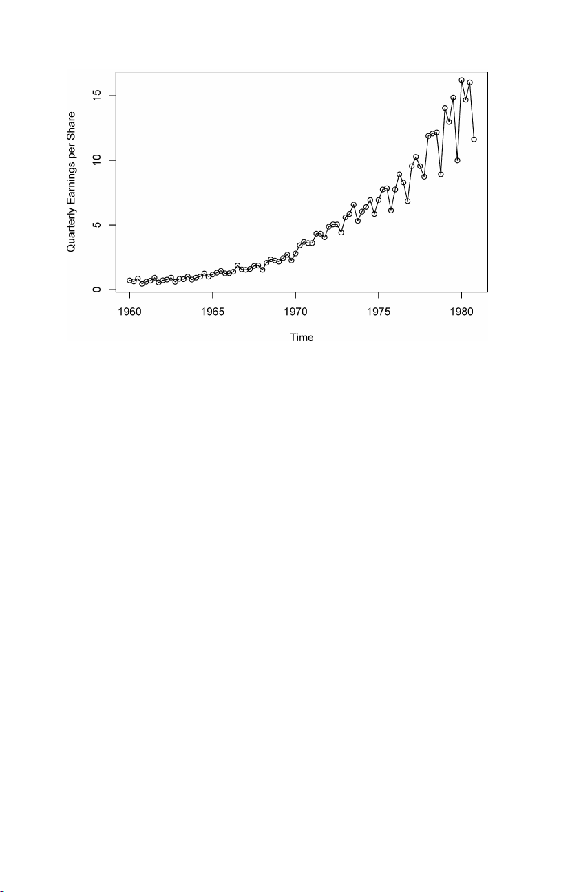
Fig. 1.1. Johnson & Johnson quarterly earnings per share, 84 quarters, 1960-I to 1980-IV.
from different subject areas. The following cases illustrate some of the com-
mon kinds of experimental time series data as well as some of the statistical
questions that might be asked about such data.
Example 1.1 Johnson & Johnson Quarterly Earnings
Figure 1.1 shows quarterly earnings per share for the U.S. company Johnson
& Johnson, furnished by Professor Paul Griffin (personal communication) of
the Graduate School of Management, University of California, Davis. There
are 84 quarters (21 years) measured from the first quarter of 1960 to the
last quarter of 1980. Modeling such series begins by observing the primary
patterns in the time history. In this case, note the gradually increasing un-
derlying trend and the rather regular variation superimposed on the trend
that seems to repeat over quarters. Methods for analyzing data such as these
are explored in Chapter 2 (see Problem 2.1) using regression techniques and
in Chapter 6, §6.5, using structural equation modeling.
To plot the data using the R statistical package, type the following:1 1 load("tsa3.rda") # SEE THE FOOTNOTE
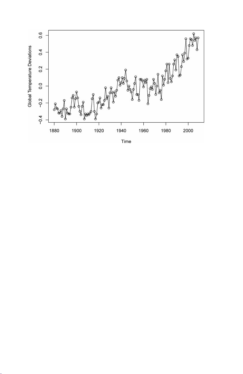
2 plot(jj, type="o", ylab="Quarterly Earnings per Share") Example 1.2 Global Warming
Consider the global temperature series record shown in Figure 1.2. The data
are the global mean land–ocean temperature index from 1880 to 2009, with
1 We assume that tsa3.rda has been downloaded to a convenient directory. See
Appendix R for further details.
1.2 The Nature of Time Series Data 5
Fig. 1.2. Yearly average global temperature deviations (1880–2009) in degrees centi- grade.
the base period 1951-1980. In particular, the data are deviations, measured
in degrees centigrade, from the 1951-1980 average, and are an update of
Hansen et al. (2006). We note an apparent upward trend in the series during
the latter part of the twentieth century that has been used as an argument
for the global warming hypothesis. Note also the leveling off at about 1935
and then another rather sharp upward trend at about 1970. The question of
interest for global warming proponents and opponents is whether the overall
trend is natural or whether it is caused by some human-induced interface.
Problem 2.8 examines 634 years of glacial sediment data that might be taken
as a long-term temperature proxy. Such percentage changes in temperature
do not seem to be unusual over a time period of 100 years. Again, the
question of trend is of more interest than particular periodicities.
The R code for this example is similar to the code in Example 1.1:
1 plot(gtemp, type="o", ylab="Global Temperature Deviations") Example 1.3 Speech Data
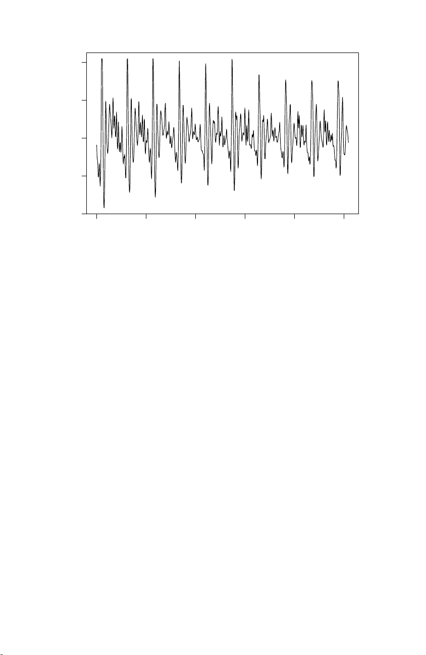
More involved questions develop in applications to the physical sciences.
Figure 1.3 shows a small .1 second (1000 point) sample of recorded speech
for the phrase aaa · · · hhh, and we note the repetitive nature of the signal
and the rather regular periodicities. One current problem of great inter-
est is computer recognition of speech, which would require converting this
particular signal into the recorded phrase aaa · · · hhh. Spectral analysis can
be used in this context to produce a signature of this phrase that can be
compared with signatures of various library syllables to look for a match. 6
1 Characteristics of Time Series 4000 3000 speech 2000 1000 0 0 200 400 600 800 1000 Time
Fig. 1.3. Speech recording of the syllable aaa · · · hhh sampled at 10,000 points per second with n = 1020 points.
One can immediately notice the rather regular repetition of small wavelets.
The separation between the packets is known as the pitch period and rep-
resents the response of the vocal tract filter to a periodic sequence of pulses
stimulated by the opening and closing of the glottis.
In R, you can reproduce Figure 1.3 as follows: 1 plot(speech)
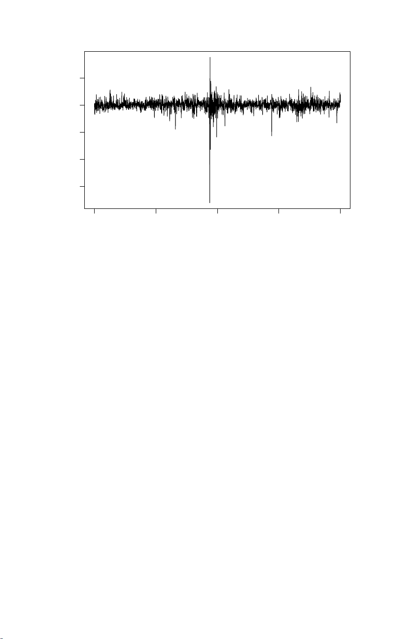
Example 1.4 New York Stock Exchange
As an example of financial time series data, Figure 1.4 shows the daily
returns (or percent change) of the New York Stock Exchange (NYSE) from
February 2, 1984 to December 31, 1991. It is easy to spot the crash of
October 19, 1987 in the figure. The data shown in Figure 1.4 are typical of
return data. The mean of the series appears to be stable with an average
return of approximately zero, however, the volatility (or variability) of data
changes over time. In fact, the data show volatility clustering; that is, highly
volatile periods tend to be clustered together. A problem in the analysis of
these type of financial data is to forecast the volatility of future returns.
Models such as ARCH and GARCH models (Engle, 1982; Bollerslev, 1986)
and stochastic volatility models (Harvey, Ruiz and Shephard, 1994) have
been developed to handle these problems. We will discuss these models and
the analysis of financial data in Chapters 5 and 6. The R code for this
example is similar to the previous examples:
1 plot(nyse, ylab="NYSE Returns")
1.2 The Nature of Time Series Data 7 0.05 ns 0.00 −0.05 NYSE Retur −0.10 −0.15 0 500 1000 1500 2000 Time
Fig. 1.4. Returns of the NYSE. The data are daily value weighted market returns
from February 2, 1984 to December 31, 1991 (2000 trading days). The crash of
October 19, 1987 occurs at t = 938. Example 1.5 El Ni˜ no and Fish Population
We may also be interested in analyzing several time series at once. Fig-
ure 1.5 shows monthly values of an environmental series called the Southern
Oscillation Index (SOI) and associated Recruitment (number of new fish)
furnished by Dr. Roy Mendelssohn of the Pacific Environmental Fisheries
Group (personal communication). Both series are for a period of 453 months
ranging over the years 1950–1987. The SOI measures changes in air pressure,
related to sea surface temperatures in the central Pacific Ocean. The central
Pacific warms every three to seven years due to the El Ni˜ no effect, which has
been blamed, in particular, for the 1997 floods in the midwestern portions
of the United States. Both series in Figure 1.5 tend to exhibit repetitive
behavior, with regularly repeating cycles that are easily visible. This peri-
odic behavior is of interest because underlying processes of interest may be
regular and the rate or frequency of oscillation characterizing the behavior
of the underlying series would help to identify them. One can also remark
that the cycles of the SOI are repeating at a faster rate than those of the
Recruitment series. The Recruitment series also shows several kinds of oscil-
lations, a faster frequency that seems to repeat about every 12 months and a
slower frequency that seems to repeat about every 50 months. The study of
the kinds of cycles and their strengths is the subject of Chapter 4. The two
series also tend to be somewhat related; it is easy to imagine that somehow
the fish population is dependent on the SOI. Perhaps even a lagged relation
exists, with the SOI signaling changes in the fish population. This possibility