Aggregate Production Planning Framework in a Multi-Product Fact - Tài liệu tham khảo | Đại học Hoa Sen

Aggregate Production Planning Framework in a Multi-Product Fact - Tài liệu tham khảo | Đại học Hoa Sen và thông tin bổ ích giúp sinh viên tham khảo, ôn luyện và phục vụ nhu cầu học tập của mình cụ thể là có định hướng, ôn tập, nắm vững kiến thức môn học và làm bài tốt trong những bài kiểm tra, bài tiểu luận, bài tập kết thúc học phần, từ đó học tập tốt và có kết quả

Ignatio Madanhire
Department of Quality and Operations Management,
University of Johannesburg, Johannesburg, South Africa
Department of Mechanical Engineering
University of Zimbabwe, rare, Zimbabwe Ha
imadanhire@eng.uz.ac.zw
Charles Mbohwa
Department of Quality and Operations Management,
Faculty of Engineering and The Built Environment
University of Johannesburg,
Johannesburg, South Africa.
cmbohwa@uj.ac.za
Abstract This study looks at the best model of aggregate
planning activity in an industrial entity and uses the trial and
error method on spread sheets to solve aggregate production
planning problems. Also linear programming model is
introduced to optimize the aggregate production planning
problem. Application of the models in a furniture production
firm is evaluated to demonstrate that practical and beneficial
solutions can be obtained from the models. Finally some
benchmarking of other furniture manufacturing industries was
undertaken to assess relevance and level of use in other furniture
firms
Keywords aggregate production planning, trial and error,
linear programming, furniture industry
I. INTRODUCTION
APID changes in global markets and international trade
has affected the management of operations in terms of
competitive positioning in the marketplace thereby posing
significant challenges for organizations. The concept of
production management has evolved beyond the scope of a
single manufacturing location. Increased competition,
coordination and control of production activities of factories
spread across regions have become more important than ever
[1]. The aggregate plan generally contains targeted sales
forecasts, production levels, inventory levels and customer
backlogs. Aggregate planning is an attempt to balance
capacity and demand in such a way that costs are minimized
Aggregate planning, being medium term in nature aims at
bridging the gap between strategic planning and operational
planning. Aggregate planning takes about 2 to 18 months [2].
During this period capacity can be managed by adding more
machines or workers, increasing working hours, reducing
workforce. Other decisions taken include changing the product
mix and to some extent the layout. In this way the company is
able to adapt to the dynamism of the market [3].
II. JUSTIFICATION
Local furniture industry has been facing challenges such as
lack of technology, obsolete equipment, long turnover time
and short product lifecycles. A solution approach to aggregate
planning problem can be used using optimization tools such as
spreadsheets and linear programming to achieve an optimum
solution. The furniture industry is a labor intensive industry
with seasonal demand in most instances.
The application of aggregate production planning in the
country is limited. The complexity of planning models is one
reason why firms do not develop advanced production
planning models. Most companies perform demand forecast,
but due to changing customer patterns, production
inefficiencies and nature of products the firms do not develop
strategies to meet the changing demands. Ad hoc strategies to
manage supply and demand are effected.
Explicit determination of the demand in terms of products
in this era is difficult therefore it fails to give the projected
load on the production facilities [4]. Aggregate production
planning is therefore, an important aspect that determines
demand in such a way as to give a clearer picture of the actual
production load. To achieve this, the products are classified
according to their size and type of operation. In this study
several aggregate planning models will be developed to find
the minimum cost for allocating the resources [5].
Adjustments are made for monitoring and control of the
industrial processes in order to respond to a changing
environment to achieve optimum performance.
III. OVERVIEW O RODUCTIOF P N
PLANNING (APP)
Manufacturing planning and control address decisions on
the acquisition, utilization and allocation of production
resources to satisfy customer requirements in the most
efficient and effective way. Typical decisions include work
force level, production lot sizes, assignment of overtime and
sequencing of production runs. Optimization models are
widely applicable for providing decision support in this
context [5]. Management makes decisions in varying
timescales and these affect overall company objectives based
on the same models.
In a highly competitive and constantly changing market
environment, it is even more important to have a high degree
of coordination between all the planning activities. It is widely
recognised that there is a great deal of potential for reducing
costs in many areas if more efficient aggregate planning
methods can be found which harmonises the system in its
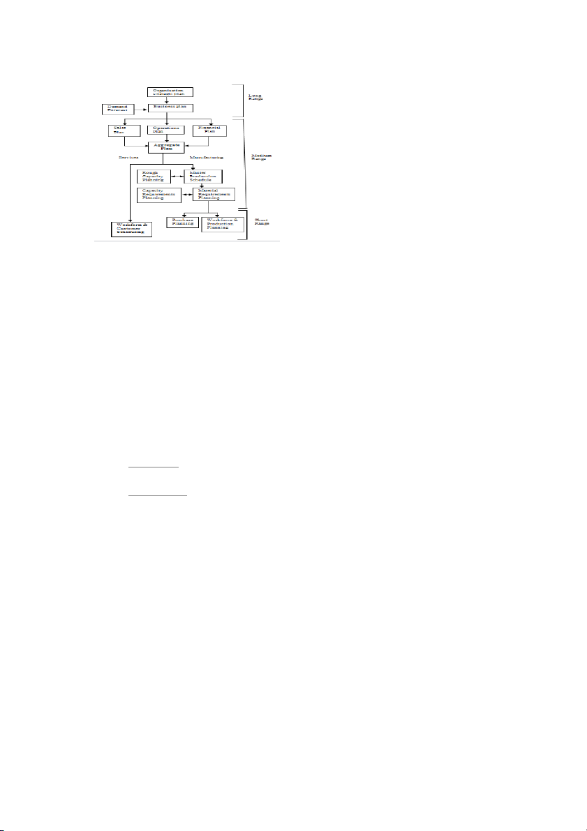
entirety[3]. The planning activity of an organisation is
illustrated in Fig 1.
Aggregate Production Planning Framework in a Multi-Product Facto
R
Proceedings of the 2015 International Conference on Industrial Engineering and Operations Managemen
Dubai, UAE, March 3 5, 2015
2531
Fig 1.Operations planning hierarchy [3]
The business plan which is long term in nature yields the
sales, operational and financial plan; these are key components
of a functioning aggregate plan. A business plan elucidates
management commitment and decision in the deployment of a
company’s resources. It sets the tone for a company’s
priorities and means of achieving the same. Essentially it is a
roadmap for business success. It highlights a well thought plan
company needs to take to reach, maintain and grow reven ue
[5].
Capacity planning is the process of determining the
production capacity needed by a manufacturing to meet
changing demands. Capacity can be defined in two ways:
design capacity and effective capacity. Design capacity is the
capacity of a process or facility as it is calculated to be whilst
effective capacity is the useful capacity of a process after
maintenance, changeover, loading and other stoppages has
been accounted for. The ratio of the actual output from a
process or facility to its design capacity yields the utilisation
of the firm [7].
Utilisation = actual output (1)
design capacity
Efficiency = actual output (2)
effective capacity
The identification of the relevant costs in aggregate
production planning is an important issue. For production
planning, firms typically need to determine the variable
production costs, including setup- related costs, inventory
holding costs, and the relevant resource acquisition costs.
Costs associated with imperfect customer service, such as
when demand is backordered should be catered for.
Planning problem always exists because there are limited
production resources that cannot be stored from period to
period. Choices must be made as to which resources to include
and how to model their capacity and behaviour, and their costs
[5] .
There is uncertainty associated with the production
function, which are uncertain yields or lead times. It is
preferable to include the most critical resource in the planning
problem for instance, a bottleneck. Alternatively, when there
is no dominant resource, then it becomes necessary to model
the resources that could limit production.
There are two types of production functions. The first
assumes a linear relationship between the production quantity
and the resource consumption. The second assumes that there
is a required fixed charge or setup to initiate production and
then a linear relationship between the production quantity and
resource usage. Related to these choices is the selection of the
time period and planning horizon. The planning literature
distinguishes between strategic and operational time periods
[8]. For strategic issues, the planner has to worry about how to
schedule or sequence the production runs assigned to any time
period. The choice of planning horizon is dictated by the lead
times to enact production and resource-related decisions, as
well as the quality of knowledge about future demand.
A.Characteristics of aggregate planning [4]
In the broad sense of the definition, the aggregate-planning
problem has the following characteristics:
A time horizon of about 12 months, with updating of
the plan on a periodic basis (conceivably monthly)
An aggregate level of product demand consisting of
one or a few categories of product the demand is
either fluctuating, uncertain, or seasonal
The possibility of changing both supply and demand
variables
A variety of management objectives which might
include low inventories, good labour relations, low
costs, flexibility to increase future output levels and
good customer service
Facilities are fixed and cannot be expanded
Aggregate planning is used in a manufacturing environment
and determines not only the overall output levels planned but
the corresponding input resources for the related products.
Various alternatives exist for matching demand with capacity.
Options which can be used to increase or decrease capacity to
match current demand include:
Hiring and laying off workers - Hiring additional workers as
needed or by laying off workers not currently required.
Overtime - This entails asking or requiring workers to work
extra hours a day or an extra day per week, firms can create a
temporary increase in capacity without the added expense of
hiring additional worker s.
Part-time or casual labour - By utilizing temporary workers
or casual labour (workers who are considered permanent but
only work when needed, on an on/call basis, and typically
without the benefits given to full/time workers) companies
reduce the salary bill significantly.
Inventory - Finished/goods inventory can be built up in
periods of slack demand and then used to fill demand during
periods of high demand
Subcontracting - Frequently firms choose to allow another
manufacturer or service provider to provide the product or
service to the subcontracting firm's customers.
2532
Cross-training - Cross/trained employees may be able to
perform tasks in several operations, creating some flexibility
when scheduling capacity.
Other methods - Among these options are sharing employees
with counter/cyclical companies and attempting to find
interesting and meaningful projects for employees to do
during slack times.
The furniture industry is a labour intensive sector thus the
workforce variable in aggregate planning needs to be
approached cautiously. Earlier studies suggested that worker
transfer between production lines is more beneficial than
hiring and firing. Worker flexibility has more impact in
aggregate planning as it enhances worker learning and reduces
labour attrition due to laying- off. Heterogeneous efficiency
of transferred workers reduces costs associated with labour
efficiency and throughput losses. Incentives, extend of
planning and the manufacturing environment which is
characterised by the tooling, work piece material,
measurement instruments and part complexity has an effect on
worker flexibility.
Demand management tends to make demand smooth and
less seasonal therefore it allows planning for constant
production throughout the year. The strategy implies that
demand be shifted from high or peak seasons to low seasons
where most firms are operating below capacity. Aggregate
Planning can be used to influence demand as well as supply.
Options exist for situations in which demand needs to be
increased in order to match capacity (supply) include [10]:
Pricing. Vary prices to increase demand in periods
when demand is less than peak.
Promotion. Advertising, direct marketing, and other
forms of promotion are used to shift demand.
Back ordering. By postponing delivery on current
orders demand is shifted to period when capacity is
not fully utilized.
New demand creation. A new, but complementary
demand is created for a product or service.
Also manufacturers and their suppliers and customers can
form partnerships in which demand information is shared and
orders are placed in a more continuous fashion.
B. Aggregate Planning Strategies
There two pure planning strategies available to the aggregate
planner are level strategy and a chase strategy. Firms may
choose to utilize one of the pure strategies in isolation, or they
may opt for a strategy that combines the two[7].
i. Level Strategy-A level strategy seeks to produce an
aggregate plan that maintains a steady production rate and
steady employment level. As demand increases, the firm is
able to continue a steady production rate, while allowing the
inventory surplus to absorb the increased demand. A level
strategy allows a firm to maintain a constant level of output
and still meet demand. This is desirable from an employee
relations standpoint.
ii. Chase Strategy-A chase strategy implies matching demand
and capacity period by period. This could result in a
considerable amount of hiring, firing or laying-off of
employees, increased inventory carrying costs and erratic
utilization of plant and equipment. The major advantage of a
chase strategy is that it allows inventory to be held to the
lowest level possible, and for some companies this is a
considerable savings. Most firms embracing the just in time
production concept utilize a chase strategy approach to
aggregate planning [8].
iii. Hybrid strategy- In some instances a combination strategy
can be found to better meet organizational goals and policies
and achieve lower costs than either of the pure strategies used
independently.
The role of aggregate planning may be described as
establishing a regime of production situations that are
achievable, controllable and utilizing available capacity.
However capacity is more expensive than inventory. It is in
capacity management that companies have the largest
potential to gain competitive advantage. For this to occur
companies need skill based competencies in aggregate
production planning system design.
C. Production costs
The objective of the aggregate planning is to minimise the
total cost of production within the planning horizon, hence
need to investigate which costs affect the total cost of
production on aggregate production and employment levels.
The following costs are included [7]:
Raw material cost
Direct payroll cost
Overtime cost
Hiring / Firing cost
Inventory / shortage cost
Direct payroll costs are calculated by taking the average
wage of worker and multiplying it with the number of each
workers employed during the period. Salaried staff and
management costs are excluded, since they are considered to
be relatively fixed during the planning horizon. Overtime costs
are calculated by multiplying the total man-months of
overtime by the regular pay and the overtime payment factor.
Hiring costs include the cost of interview test, medical
examination and training. Termination benefits, gratuities, and
negative impact on employees’ morale all help determine the
firing cost. Inventory costs are the sum of holding or storage
cost, interest on tied capital and depreciation. Shortage costs
are due to the potential loss of the customers and the negative
effect on the reputation of the firm.
The complexity of models coupled with the lack of
adequate data makes firms avoids using aggregate production
planning (APP) models. Also the use of spread sheet
modelling and trial and error approach can create useful but
simple solutions to APP models. Studies have suggested using
the learning curve effect on the model where the user can find
the least cost plan under different learning rates. In this study
trial and error methods will be constructed and Lindo software
will be used to solve a mixed integer linear programming
problem [9].
2533
IV. R ESEARCH DESIGN
Aggregate production planning (APP) determines the
capacity a company needs to meet its demand over a certain
period of time varying from two to eighteen months. During
this time frame it is not feasible to increase capacity by
building new facilities or purchasing new equipment, however
it is feasible to adjust employee level, add extra shifts,
outsource, use overtime or change inventory levels.
A.Model development
The basic model to minimize the total cost is developed as
shown below.
Minimize:
Total production cost over planning horizon
= Raw Material Cost + Payroll cost + Hiring cost + Firing
cost + Overtime cost + Inventory cost + Shortage cost
B. Aggregate planning techniques
The techniques range from simplistic, graphical methods to
the highly sophisticated linear decision rule and the
parametric production-planning method. The most
sophisticated techniques can be considered as optimizing,
search, heuristic, and dynamic methods. Within each of these
categories are numerous alternative approaches, resulting in an
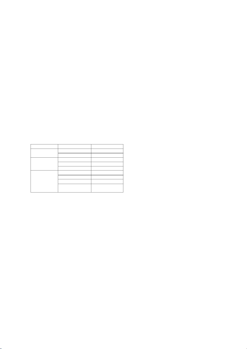
abundance of theoretical solution procedures. Table I gives
some of the common techniques used [3].
TABLE I
AGGREGATE PLANNING TECHNIQUES
Classification
Type of Method
Type of Cost Structure
Feasible Solution
Methods
Barter
General/not explicit
Graphic/tabular
Linear/discrete
Mathematically
Optimal Methods
Linear programming models
Linear/continuous
Transportation models
Linear/continuous
Linear decision rules
Linear/quadratic/continuous
Heuristic decision
procedures
Simulation search procedure
General/explicit
Management coefficients
Not explicit
Projected capacity utilisation
Not explicit
Parametric production
planning
Quadratic/not specified
Informal techniques: These approaches consist of developing
simple tables or graphs which enable planners to compare
projected demand requirements visually with existing
capacity, and this provides them with a basis for developing
alternative plans for achieving intermediate-range goals.
Trial and error method[1]: It is used to solve aggregate
production planning since this method is easy to understand
and it is used to convey planning details without getting
involved with mathematical detail. It is used to develop
manufacturing plans, determine cost and feasibility of each
plan and selection of the lowest cost plan among feasible
alternatives. Trial and error methods follow the steps below:
-Prepare an initial aggregate plan on the basis of forecasted
demand and establish guidelines
-Determine if the plan is within capacity constraints. If not
revise until it is.
-Determine the costs of the plan
-Transform the production plan to lower costs.
-Continue the process until a satisfactory plan is developed
-Perform sensitivity analysis to evaluate the effect of changes
in such parameters as the carrying cost rate, the costs of hiring
and firing and demand
-Track the plan (compare actual results to the planned results)
Two extreme plans i.e. the level production and the chase
strategy are developed first. Compromises within these
extremes are then developed and evaluated.
Linear programming(LP): It is concerned with maximisation
and minimisation of a field of a linear objective function in
many variables subject to equality and inequality constraints
for instance the function may seek to minimise the cost of
hiring/firing workers, holding inventory. The problem consists
of selecting the values for several non-negative variables so as
to minimize a linear function (the total relevant costs) of these
variables subject to several linear constraints on the variables.
An important benefit of a linear programming model is the
potential use of the dual solution to obtain the implicit costs of
constraints such as the maximum allowable inventory level.
An algorithm called the simplex method was develope to find d
an optimal solution to linear programming models [5]. The
optimal solution must be a vertex of the feasible region. All
that is needed is to find the vertices with the most favourable
value of the objective function in order to identify all optimal
solutions.
Goal programming [4]: The objective of aggregate production
planning is either to maximise profit or minimise cost. In
linear programming it is formulated as a single objective.
Whereas, in real life there are multiple objectives to a
problem. Problems involving multiple objectives can be
solved using linear programming where one objective is
optimised and the others are considered in the constraints.
In goal programming the concept of optimum solution of LP
problems is substituted by a satisfactory and non-dominated
solution In goal programming the levels of . pre-emptive
achievement are provided, priorities to goals are determined.
More important goals are optimised before low level goals are
considered. Several solutions can be obtained and the best
solution will depend on the priority assigned to each goal.
Linear decision rule: When various costs can be
approximated by linear and quadratic functions it turns out
that the decision rules for setting the workforce sizes and
production rates are of simple linear form. The objective of
this method is to derive linear equations or decision rules
which can be used to specify the optimal production rate and
workforce level over some prescribed production planning
horizon. The linear decision rule has been shown to lead
to costs significantly lower than those encountered under
the existing management procedure. There is no easy way of
including constraints on the inventory or production levels.
Management coefficients approach: It assumes that managers
behave in a rational fashion. Past behaviour of managers is
used to estimate the unknown coefficients in plausible
decision rules. The strong point of this method is that it has
intuitive appeal to management. This makes implementation
2534
considerably easier than in the case of a sophisticated
mathematical decision model. The assumption that the past is
a good description of the future may prevent the manager from
quickly adapting to new conditions in a rapidly changing
competitive environment [3].
Simulation search procedures: The approach here is that a
closed-form mathematical solution cannot be obtained when
the model is made truly representative of the prototype
situation. Therefore, a mathematical model is developed which
represents quite accurately the actual cost functions and
constraints. Then, by a trial and error procedure, the variables
are varied until there results no further reduction in the total
relevant costs. A computer is often used to facilitate this
search procedure. These procedures include search decision
rule, parametric production planning, and a manual simulation
approach
Parametric production planning: This model provides
another angle in production planning. Optimization guarantee
is relaxed and two rules in terms of four parameters are
created. The first rule gives the size of workforce and the
second the production quantity. The four parameters take
values between 0 and 1 [7]. The combinations are tested and
used to establish the total cost.
The selection of aggregate production planning strategy
depends on several factors like demand distribution,
competitive position of the company, the product cost
structure and the product line. In this thesis quantitative
techniques will be used to aid the decision making.
V. FURNITURE OMPANY OVERVIEWC
Spring Master Company is a wood furniture manufacturing
company located in Harare with two factories in two different
operating sites. The main plant deals with hardwoods like
teak, oak and mahogany, while the second plant mainly
manufactures pine furniture. The areas of analysis were the
production departments/sections namely: the breakdown
section, machine shop, sub-assemblies, carving, and
upholstery section, assembly section, finishing section,
final fitting section and the warehouse. The company
manufactures furniture for the office, bedroom, lounge, dining
and occasional. The other items include chest of drawers, TV
stands, TV cabinets, wine racks, hall tables and mirrors among
other things. supplies the local (93%) and export (7%) It
markets but the bulk of their products satisfies the local
market. The firm supplies individual customers, government
departments, retail shops, companies among a host of its
clientele base.
VI. R ESEARCH FINDINGS
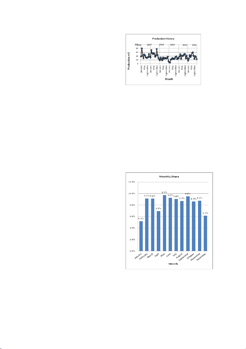
The production performance for the plant from January
2006 to December 20 is given in Fig 11 2
Fig 2.Production history
The pre-2008 era has the highest production figures this ing be
attributed to prevailing disposable incomes, stable
employment rates and sound capital equipment. Thereafter
post dollarization era posed a range of challenges in
equipment capitalisation, job redundancy and cost
minimisation in addition to depressed macro and micro
economic environments. The low activity in December and
January of every year can be attributed to the short production
and selling time as it is annual festive season break and
maintenance shutdown period .
A. Demand forecast
The plant at its peak used to handle a capacity of 80m per
3
month but this has since been reduced due to aging equipment,
depressed market conditions and employee turnover. In this
study the maximum plant capacity was estimated at 60m per
3
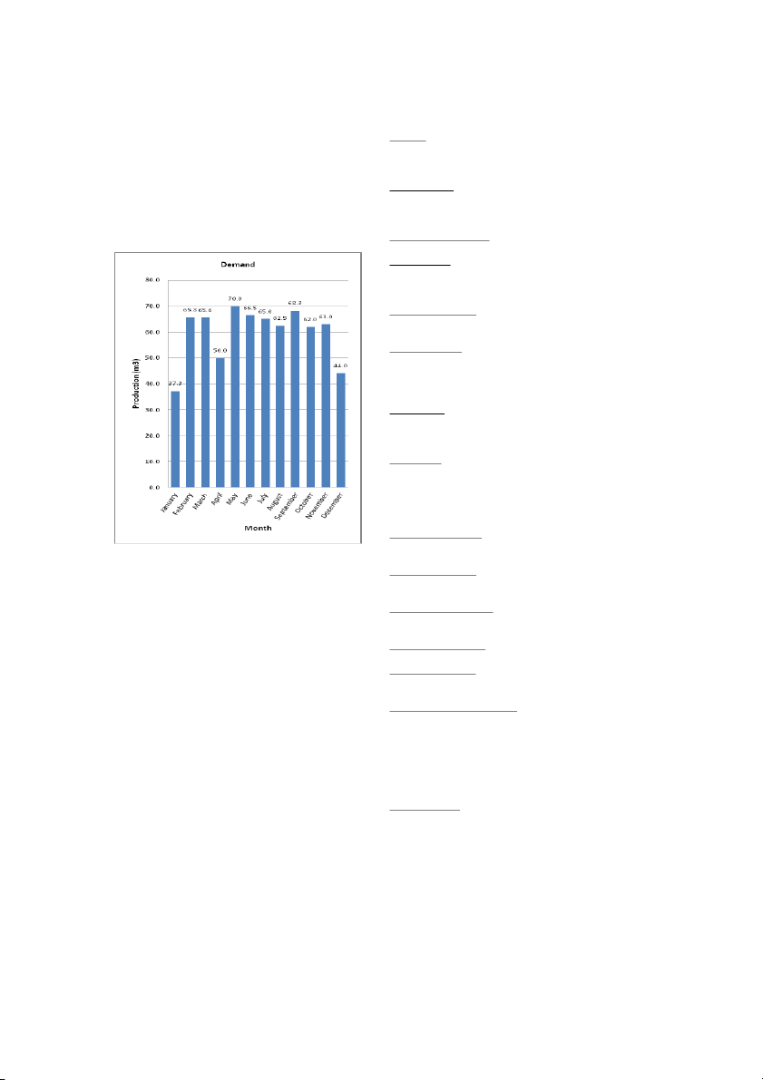
month. The data was analysed for seasonality in a year and the
monthly contribution to production was noted. The graph
below shows the monthly contribution towards production
from January 2006 to December 2011.
2535
Fig 3.Average monthly contributions towards annual
production
The monthly share was used to estimate the production for the
month. For analysis it was not unusual to note that the January
and December had the lowest figures. This can be attributed to
the short operating times. It was also seen that April and
August had significant drops in production (6.9% and 8.7%
respectively). Possible justification for this might include
significant holiday breaks and hence a decline in the output.
The demand forecast for the months is shown graphically
below.
Fig 4.Demand
B. Aggregate production planning model
The model to be developed aims at reducing production costs.
It will also analyse chase and level demand strategies. The
strategies will be used to come up with a hybrid strategy that
reduces the costs even further. The results will be compared
against computed results from the linear programming model.
The linear programming model will be used to develop a
model to enhance the decision making process for
management.
Assumptions
-All furniture will be grouped under the five product families
office, bedroom, dining, lounge and occasional
-Demand is in USD terms and the company aims at achieving
60m
3
of production. 42% being office, 18% dining, 16%
occasional, 12% lounge, 12% bedroom. (from past financial
records)
-Capacity of the firm is 60m per month.
3
-Beginning inventories are estimated to be are one fourth of
the capacities of the firm
-Beginning backorder value is zero
-Inventory level changes at the beginning of every month by
the amount that is transferred from the previous month
Data
Demand -The demand for a given month is calculated from
the annual target and multiplied by the monthly contribution
towards the target based on 5 year analysis.
Working days -Working days per month vary in months with
long holidays and breaks (January, April, August and
December). On average they are assumed to be 22.
Working hours per day: 9.5
Regular wage: The minimum wage according to the National
Employment Council (NEC) ruling in the furniture industry
will equal $265.
Overtime limitation: There is a limit of four weekends per
employee for overtime which amounts to 8 days per month
Overtime wage: According to the Labor law the wage payable
for each hour of overtime paid by increase the amount
overtime is paid increasing the amount of normal work wage
per hour by fifty percent
Hiring cost: According to the World Bank Reports Doing
Business the average hiring cost per worker is equal to 6% the
gross salary (nationmasters.com)
Firing cost: According to the same report, the firing cost can
be estimated to be 29.3 weeks of wages. However the cost
actually depends on the amount of time a worker has been
employed. In this study the firing cost will be calculated by
multiplying the salary by 7.3.
Maximum Inventory: Maximum allowable inventory 50% of
the capacity of the firm
Minimum Inventory: Minimum inventory level One tenth of
the capacity of the firm
Inventory Holding Cost: The inventory holding cost is 2% of
the market prices of the products per month.
Raw material cost are: 30% of the product cost
Capacity utilization of the Spring Master Company factory is
averaging 54% for 2011
Maximum number of workers: Although the workers vary with
the chosen strategy but based on the company capacity of
80m
3
per month and the capacity of employee to be 0.3m per
3
month the number of shop floor workers required is 200.
However since the capacity utilization is hovering at 54% the
company will need at least 108 workers as the company will
not function at full capacity every month.
Backorder cost: This cost arises when the demand cannot be
met in the period it is supposed to be. It can be calculated as
equal to 0.75 times the product cost.
2536
Lost sales cost: Although it is difficult to quantify this cost can
be quantified base on assumptions. This cost reflects the losses
of sales revenue and goodwill when the producer is not able to
fulfill demand and it is given as 1.4 times the product cost.
Subcontracting cost: Subcontracting cost should be treated as
a necessity applied despite its unfavorable costs otherwise all
companies would opt to subcontract instead of producing
themselves. For this reason subcontracting cost will be higher
than the total cost /unit but will be lower than the lost sales.
Subcontracting cost is assumed to be cost 1.2 times the
product cost.
B. Linear programming model
The following model is based on the Lindo Systems
optimisation. Many LP models contain hundreds of
constraints and decision variables. The objective of the model
is to minimise all related costs in the setting up of an
aggregate plan. Such costs include raw material cost, labour
costs i.e. regular, overtime, hiring and firing costs, inventory
costs, backorder, subcontracting and lost sales cost.
Model parameters
Products j: 1… N N =5
Periods t: 1… T T=12
N = 1 dining furniture
2 lounge
3 -- bedroom furniture
4 -- occasionals
5 -- office furniture
T= 1 -- January…………..T = 12 for December
Parameters
D
tj
-- demand forecasted for product j in period t
m hours required to produce 1m3 of product j in period t
tj--
OTCAP overtime production hours for product j in period t
tj
WRCAPMAX maximum number of workers for product j
tj
in period t
WRCAPMIN minimum number of workers for product j in
tj
period t
w raw material cost per unit of product j
j
i - inventory carrying cost per unit of product j
j
b
j
backorder cost per unit of product j
l lost sales cost per unit of product j
j
MINI minimum quantity of inventory per product j
j
MAXI maximum quantity of inventory per product j
j
--
MAXBO upper limit for the amount of product j that can be
j
--
backordered
IB
j
initial value of inventory
BB
j
initial value of backorder
WH number of regular per worker in period t
r- cost of man hour regular time
o- overtime cost per man hour
h- cost of hiring a worker
f-cost of firing a worker
Decision variables
X
tj
units of product j to be produced in period t
IN
tj
quantity of product j to be kept in inventory in period t
BO
tj
quantity of product j to be backordered in period t
LS
tj
quantity of product j which the firm loses in in sales in
period t
OT
tj
man hours of overtime labour used in period t for
product j
WR
tj
number of workers for product j in period t
RH
t
-- regular man hours of product j in period t
HR
t
number of workers hired in period t
FR
t
number of workers fired in period t
Model
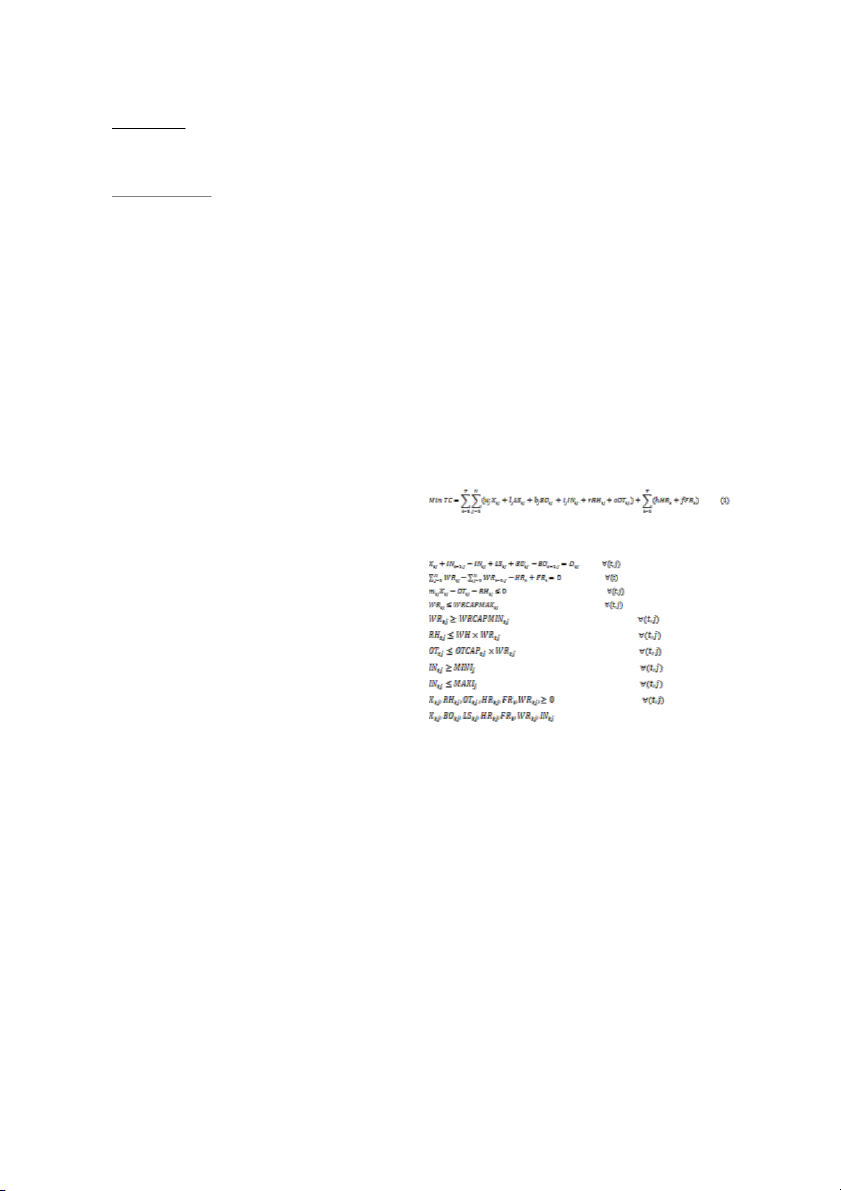
The objective of the company is to minimise total costs and
the model can be constructed as follows
Constraints
(2)
(3)
(4)
(5)
(6)
(7)
(8)
(9)
(10)
(11)
are integer values
The LINGO 13.0 model was constructed and the results are
given. Equation 2 is a constraint that ensures that the
production quantities, backordered quantities and lost sales do
not exceed the total demand quantity. Equation 3 4 and 6 are ,
constraints about the number of workers. Equation 4, 7 and 8
are constraints about regular and overtime working hours.
Equation 9 and 10 are inventory limiting models.
C. Application of trial and error methods
Application for different strategies will be done with a view
of comparing results. This was covered in conjunction with
other evaluation methods.
D. Chase strategy
2537
Chase strategies entail production at a rate in unison with
demand. The strategies available include changing the
workforce level. The strategy keeps the maximum workforce
at 200 which is enough to meet maximum demand at the
current production levels. The minimum required level of
workforce is 93. The extra manpower is hired and laid off as
and when necessar y.
In this strategy a workforce size of 108 is needed at the current
utilisation levels of around 54%. The minimum number of
workers required is 93 and the cost of this strategy amounts to
$3 439 798. This can be attributed to the failure of this
strategy to fully meet demand as can be seen by lost sales in
all the months of year except January and December. There is
a limit on the amount of production achieved by overtime as
this equates to 8 days per month and in most cases these are of
less working time than regular days. In the analysis 8 working
hours were assumed.
Subcontracting is used where the companies resources
cannot meet the expected demand and in this case in the
months of February up to December. Subcontracting has the
benefits that the company is able to let another company
produce at a price lower at or at par with the company prices
and there are significant benefits that may accrue like labour
savings and storage of inventory. The costs of the different
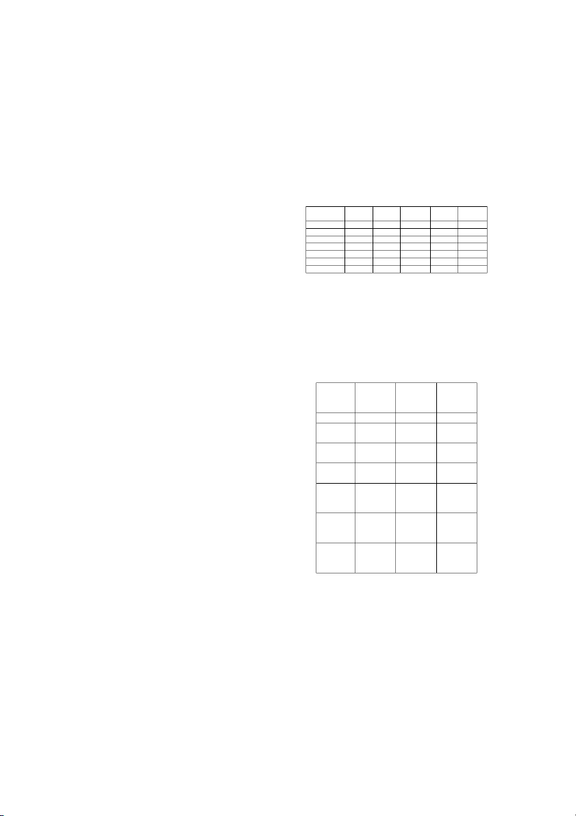
strategies are shown in the Table 2.
E. Level
The level strategy employed 200 workers producing 60m
3
of products per month. The advantage of using this strategy
for Furniture Company is that the first and last months of the
year can be used to build stocks that might be used during
periods of peak demand. The total cost for this strategy is $ 2
095 254. Labour cost and inventory holding cost for this
strategy are significant factors that contribute to the total
product cost.
F. Mixed
Analysis of all strategies shows that the level strategy can
be used to reduce costs even further by utilising the
backordering process where delivery to customers is
postponed until production can match demand yields reduced
cost. The total cost for this strategy amounts to $2 049 681.
There is a significant backordering cost associated with this
strategy in comparison with the level strategy.
G. Lingo solution
The total cost computed by the LINGO 13.0 model is $1
878 384 which is a slightly better solution as compared to the
trial and error methods. LP models can be practical and
beneficial once models have been constructed. Constraints are
easily applied to the formulated model.
According to the generated solution of the linear production
model a workforce of 108 people is enough to cater for the
whole year with variation in demand being met using
inventory and over time. Most of the demand is met within the
year so there is backordering and lost sales cost. Trial and
error methods also give a good approximation of the
production costs and cannot be totally ignored. However in
real life situation many objectives have to be settled at once
not just the cost aspect to it. For instance it might be necessary
to reduce cost, reduce the hiring and firing rates and the cost
limits. Linear programming can be modelled to cater for the
underachievement or overachievement of certain goals like
inventory levels, firing and hiring thresholds and the ceiling
production cost targeted.
VII. A DATA NALYSIS
A. Comparison of strategies
TABLE II
COMPARISON OF STRATEGIES
Hire/Fire
($)
Overtime
($)
Subcontract
($)
Level ($)
Mixed ($)
1 252 690
1 497 078
1252690
1 04 000
1 252 690
1 038 853
686 880
509 494
636 000
636 000
0
0
4314
0
139 425
0
1245753
0
0
0
10 087
10 087
10 087
65 142
21 66
0
0
593 435
0
0
2 301 630
3 439 798
2 370 021
2 095 254
2 049 681
B. Cost analysis
The current cost analysis at Spring Master Company shows
that the cost of sales for the 2011 trading year was $ 1 965 456
against a figure of $ 1 410 814 for 2010. However the total
annual production for 2011 was 446 m against a figure of
3
464m
3
for 2010. The cost of sales can be broken down into the
following categories as depicted in the Table III.
TABLE III
COST OF SALES ANALYSIS
2011
2010
Average
Percentage
Contribution
Cost of sales
$ 1 965 456
$ 1 410 814
Direct
material cost
49.8%
49.8%
49.8%
Direct staff
costs
40.4%
41.8%
41.1%
Maintenance
costs
6.8%
7.0%
6.9%
Direct
Operating
Expenses
7.3%
8.6%
8.0%
ISO and
Quality
Costs
0.3%
0.2%
0.3%
Direct
overheads
costs
-4.7%
-7.4%
-6.0%
From the above analysis and the fact that the computed results
from the trial and error methods and the linear programming
model exclude maintenance, quality and direct operating
expenses. The cost of sales in the table can then be adjusted to
exclude these costs to enable a fair comparison.
2538
TABLE IV
OST OMPARISONC C
Cost ($)
Quantity
produced
(m
3
)
Number
of
employees
Current
1 786 389
446
194
Previous year (2010)
1 282 279
464
179
Trial and error
2 049 681
720
200
Linear programming
1 878 384
720
108
From Table 4 it can be appreciated that the cost of sales has
gone up since the previous year i.e. 2010 this can be attributed
to the increase in cost of raw materials, overheads and direct
labour costs. An accurate assessment of the cost can be based
on the parameter presented in Table V below
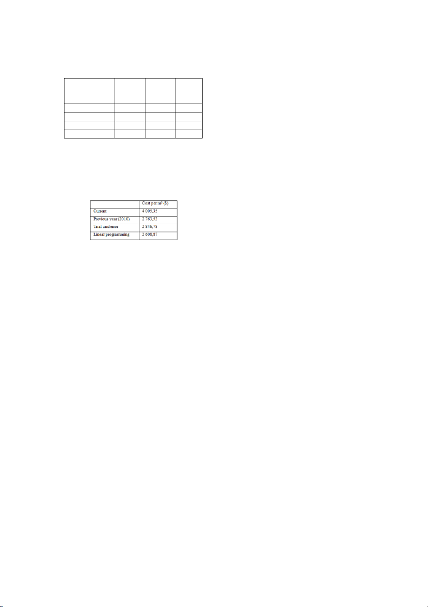
TABLE V
COST PER UNIT
The cost per cubic metre is spiralling and it will balloon if left
uncontrolled. It is crucial that Adam Bede ascertain a targeted
cost of sales then work around it in monitoring and
eliminating deviations. The analysis shows an average of $3
384,44 per cubic metre over the past two years. Adopting
aggregate production planning process yields a cost reduction
of 16% per m on the spread sheet model and 23% on the use
3
of linear programming models.
C. Throughput
The plant currently process 1.76 cubic metres of timber
product into the warehouse every day. However with each
man capable of 0.3m per month this falls short of
3
expectations. This will ultimately yield much lower
production as reduced speeds; minor stoppages and plant
unavailability weigh in. A target of 60m per month which the
3
proposed model assumes is realistic and achievable judging
from past targets and production figures. The aggregate
production planning strategies proffered are in agreement with
this production target. The daily target becomes 2.73m of
3
timber/furniture into warehouse. This makes an increase of
0.97m
3
. In the event of failure by employees to meet the daily
demand it can be augmented by overtime after normal hours
or during weekends.
D. Benchmarking
It was observed that most furniture industries are family
owned businesses where decisions are centrally made. The
type of management does not allow essential components of
aggregate planning like demand forecast and re-planning to be
carried out effectively. Ad hoc strategies by default tend to be
used in meeting demand. From interviews it was highlighted
that there is an insatiable demand for furniture products such
that there little use of aggregate production strategies. It was
also pointed out that raw material especially timber is being
sourced from non-sustainable local sources such that in the
long run alternative sources of timber have to be explored.
This will have adverse effects on the production cost and
judging from the influx of cheap foreign furniture products
mainly from Asia, it becomes imperative companies minimize
costs. It was also evident that the companies specialize in
either hardwood or softwood products. Each company has a
niche market that it capitalizes on to improve revenue.
The study revealed that no furniture company utilizes
aggregate production planning philosophy in its entirety.
Market analysis is done either to position the company with
competitors or exploit changing customer tastes. It was also
seen that workers in most factories all factories were above
130. Obsolete infrastructure does not impede furniture
manufacturing but it tends to shift production from being
semi-automatic to completely manual which ultimately results
in many manual activities.
Demand for furniture was viewed as fluctuating and all
companies assessed produce to match demand. The companies
utilize overtime, casual labor and cross training or multi
skilling among the preferred options to meet demand. It was
also evident that some companies use advertising mainly as a
brand awareness campaign to improve revenue. Changing
prices proved popular in the strategies used to match
production capacity to demand. Lead times of four weeks on
average was utilized by most companies.
VIII. RECOMMENDATIONS
Mathematical techniques will likely have to be balanced
with managerial judgment and experience. Whilst it might
prove attractive mathematically for example in cases where
firing employees makes sense, managerial experience might
show decreasing productivity and worker attrition which
models might fail to expose in each planning horizon.
Managers act in a rational manner and will tend to make
decisions that reduce exposure to risk; this makes strategies
like hiring and firing or subcontracting difficult to effect even
though theoretically they make business sense.
There is a tendency to blur the distinction between
production planning and production scheduling. Planning
precedes scheduling. Aggregate planning in particular is
applied to a group of products and therefore does not yield
detailed planning and scheduling information. It helps bridge
the gap between strategic and operational planning.
The case study company, from analysis can taper into this
strategy to realize full benefits that accrue if a systematic
aggregate production planning model is utilized. From the
models derived the following recommendations are suggested.
Spring Master Company should adopt a hybrid system
preferably that harness the benefits of level and chase demand
strategies. The use of a steady workforce level that keeps
production at a consistent rate should yield tangible benefits to
the company. The trial and error method suggested offers a
cost reduction of 16% per cubic metre and the linear
programming model pushes it further to 22%. In periods of
slack demand or reduced production e.g. in January, April and
December the company can systematically utilise these
months to send employees on vacation. A system of
2539
annualised working hours is also an attractive proposition as
not all workers are needed in the first and last months of the
year. Workers can also be reduced for months like April and
August. In this regard workers who had worked overtime in
periods of peak demand can be asked or required to work less
during this period. The workers should not include skilled
labour as this creates dissension and aid high employee
turnover. Skilled workers tend to engage themselves in gainful
activities outside the working environment; giving them
periods of extended breaks might prove counterproductive.
The organization should cross train its employees to handle a
variety of orders and engage in more frequent re-planning
during the year. In addition management should carefully
analyse their decision rules for aggregate planning before the
implementation.
It should also revise its corporate strategy to incorporate a
manufacturing unit strategy that outlines the company’s
preferred order winning criteria. The order winning criteria is
based on the need for companies to turn orders into tangible
business. It premises on the need to use time, cost and quality
aspects to a company’s advantage. Quality has always been a
mainstay of Spring Master operations but if the cost and
delivery speed angle is fully utilised, the company can reap
outstanding rewards. Furniture industries tend to be more
specialised and orders tend to be more unique and customer
specific. In every furniture firm they are products that are well
known and are considered a flagship of the organisation.
Spring Master office furniture is well known and preferred
locally. Spring Master can shift from a make to order
philosophy to a make to stock and harness the benefits that
accrue due exploitation of delivery speed. This philosophy can
be coupled with pro-activeness in managing the supply chain.
Managing demand through promotions and advertising will
ease production loading and smooth demand.
IX. C ONCLUSION
Furniture industry is an industry where manufacturing
companies do not prefer to use aggregate production planning
techniques. The reasons for their poor usage in this particular
sector include their complexity and time needed to develop
and refine models. The use of models in some instances is
synonymous with qualified engineers as it needs an extensive
mathematical background. The Zimbabwean furniture industry
is dominated by family owned businesses where decision
making is highly centralised. The decisions from sales,
production and accounting are mainly done by a few dominant
figures with the rest assuming supervisory and policing roles.
In this work it was shown that trial and error methods
provide a good approximate on its use and application in an
industrial set-up. Cost savings of at least 16% per cubic metre
were observed and throughput of 2.27m per day was
3
proffered as attainable. The Zimbabwean furniture industry
lacks latest technology and these methods provide helpful
production plans. Most developed software on the other hand
provide easy to use solutions which can be more exact and
accurate than trial and error methods proposed (cost savings of
22% were realised using the linear programming model).
Furniture industry is a labour intensive sector, therefore not all
proposed theoretical solutions such as hiring and firing and
subcontracting are beneficial to the sector.
X. F RURTHER ESEARCH
The emergence of improved hierarchical production planning
has proved to be popular in the field of aggregate planning.
This phenomenon is providing useful insights in the
production planning process. Aggregate production planning
models are formulated analytically and this often results in
large mathematical programming models. As computational
models become excessive and large, it is impossible to
develop optimal solutions. Decomposition techniques are one
way of solving large scale models.
R EFERENCES
[1] Bitran, G. R, Tirupati, D (2011) Hierarchical Production Planning
[2] Dileepan P and Ettikin L.P (2010), Learning: the missing ingredient in
production planning spreadsheet models, Inventory Management Journal
20(3) 32- 35
[3] Graves S.C(2006), Manufacturing Planning and Control Massachusetts
Institute of Technology
[4] Hax, A. C, Meal H. C(2007), Hierarchical Integration of Production
Planning and Scheduling, Management Sciences, Vol. 1: Logistics, New
York, Elsevier, pp. 53-69.
[5] Jones C. H (2005), Parametric Production Planning, Management
Science 11(13), pp 843-866
[6] Konje P, Zimbabwe Furniture Brief, Zimtrade Publication, 2011
[7] Penlensky R, Srivastava R (2011), Aggregate Production Planning using
spreadsheet software, Production Planning and Control 5(6) 524- 532
[8] Silver, E.A.(2003), Medium-range aggregate production planning: state
of the art, Production and Inventory Management, First Quarter, pp. 15-
39.
[9] Techawiboonwog A, Yenradae P {2009), Aggregate Production
Planning with workforce transferring plan for multiple product types,
Production Planning and Control journal pg 14(5) 447-458
AUTHORS
Ignatio Madanhire is a PhD student in Engineering
Management at the University of Johannesburg. He is also a
lecturer with the Department of Mechanical Engineering at the
University of Zimbabwe. He h research interests in as
engineering management and has published works on cleaner
production in renowned journals
Charles Mbohwa is a Professor of Sustainability Engineering
and currently Vice Dean Postgraduate Studies, Research and
Innovation with the University of Johannesburg. He is a keen
researcher with interest in logistics, supply chain management,
life cycle assessment and sustainability, operations
management, project management and engineering /
manufacturing systems management. He is a professional
member of mbabwe Institution of Engineers (ZIE) and a Zi
fellow of American Society of Mechanical Engineers
(ASME).
.
2540
| 1/10

Preview text:

Proceedings of the 2015 International Conference on Industrial Engineering and Operations Managemen
Dubai, UAE, March 3 5, 2015
Aggregate Production Planning Framework in a Multi-Product Facto Ignatio Madanhire Charles Mbohwa
Department of Quality and Operations Management,
University of Johannesburg, Johannesburg, South Africa
Faculty of Engineering and The Built Environment University of Johannesburg,
Department of Mechanical Engineering Johannesburg, South Africa.
University of Zimbabwe,Harare, Zimbabwe cmbohwa@uj.ac.za imadanhire@eng.uz.ac.zw
Abstract This study looks at the best model of aggregate planning models. Most companies perform demand forecast,
planning activity in an industrial entity and uses the trial and but due to changing customer patterns, production
error method on spread sheets to solve aggregate production inefficiencies and nature of products the firms do not develop
planning problems. Also linear programming model is strategies to meet the changing demands. Ad hoc strategies to
introduced to optimize the aggregate production planning manage supply and demand are effected.
problem. Application of the models in a furniture production
firm is evaluated to demonstrate that practical and beneficial
Explicit determination of the demand in terms of products
solutions can be obtained from the models. Finally some in this era is difficult therefore it fails to give the projected
benchmarking of other furniture manufacturing industries was
load on the production facilities [4]. Aggregate production
undertaken to assess relevance and level of use in other furniture planning is therefore, an important aspect that determines firms
demand in such a way as to give a clearer picture of the actual
production load. To achieve this, the products are classified
Keywords aggregate production planning, trial and error, according to their size and type of operation. In this study
linear programming, furniture industry
several aggregate planning models wil be developed to find
the minimum cost for al ocating the resources [5]. I. INTRODUCTION
Adjustments are made for monitoring and control of the
APID changes in global markets and international tradie
n dustrial processes in order to respond to a changing
Rhas affected the management of operations in terms oefn vironment to achieve optimum performance.
competitive positioning in the marketplace thereby posing III. OVERVIEW OF PRODUCTION
significant challenges for organizations. The concept of
production management has evolved beyond the scope of a PLANNING (APP)
single manufacturing location. Increased competition, Manufacturing planning and control address decisions on
coordination and control of production activities of factoriest he acquisition, utilization and al ocation of production
spread across regions have become more important than eve
r re sources to satisfy customer requirements in the most
[1]. The aggregate plan general y contains targeted sale
e sff icient and effective way. Typical decisions include work
forecasts, production levels, inventory levels and custome
f ro rce level, production lot sizes, assignment of overtime and
backlogs. Aggregate planning is an attempt to balance
s equencing of production runs. Optimization models are
capacity and demand in such a way that costs are minimized
widely applicable for providing decision support in this
context [5]. Management makes decisions in varying
Aggregate planning, being medium term in nature aims at
bridging the gap between strategic planning and operationta i l
mescales and these affect overal company objectives based on the same models.
planning. Aggregate planning takes about 2 to 18 months [2].
During this period capacity can be managed by adding more In a highly competitive and constantly changing market
environment, it is even more important to have a high degree
machines or workers, increasing working hours, reducing
workforce. Other decisions taken include changing the produc
o tf coordination between al the planning activities. It is widely
recognised that there is a great deal of potential for reducing
mix and to some extent the layout. In this way the company is
able to adapt to the dynamism of the market [3].
costs in many areas if more efficient aggregate planning
methods can be found which harmonises the system in its
entirety[3]. The planning activity of an organisation is II. JUSTIFICATION il ustrated in Fig 1.
Local furniture industry has been facing challenges such as
lack of technology, obsolete equipment, long turnover time
and short product lifecycles. A solution approach to aggregate
planning problem can be used using optimization tools such as
spreadsheets and linear programming to achieve an optimum
solution. The furniture industry is a labor intensive industry
with seasonal demand in most instances.
The application of aggregate production planning in the
country is limited. The complexity of planning models is one
reason why firms do not develop advanced production 2531
preferable to include the most critical resource in the planning
problem for instance, a bottleneck. Alternatively, when there
is no dominant resource, then it becomes necessary to model
the resources that could limit production.
There are two types of production functions. The first
assumes a linear relationship between the production quantity
and the resource consumption. The second assumes that there
is a required fixed charge or setup to initiate production and
then a linear relationship between the production quantity and
resource usage. Related to these choices is the selection of the
time period and planning horizon. The planning literature
distinguishes between strategic and operational time periods
[8]. For strategic issues, the planner has to worry about how to
schedule or sequence the production runs assigned to any time
period. The choice of planning horizon is dictated by the lead
times to enact production and resource-related decisions, as
wel as the quality of knowledge about future demand.
Fig 1.Operations planning hierarchy [3]
The business plan which is long term in nature yields the A.Characteristics of aggregate planning [4]
sales, operational and financial plan; these are key components
In the broad sense of the definition, the aggregate-planning
of a functioning aggregate plan. A business plan elucidates
pr oblem has the fol owing characteristics:
management commitment and decision in the deployment of a  A time horizon of about 12 months, with updating of
company’s resources. It sets the tone for a company’s
the plan on a periodic basis (conceivably monthly)
priorities and means of achieving the same. Essential y it is a  An aggregate level of product demand consisting of
roadmap for business success. It highlights a wel thought plan
one or a few categories of product – the demand is
company needs to take to reach, maintain and grow revenue
either fluctuating, uncertain, or seasonal [5].
 The possibility of changing both supply and demand variables
Capacity planning is the process of determining the
production capacity needed by a manufacturing to meet  A variety of management objectives which might
include low inventories, good labour relations, low
changing demands. Capacity can be defined in two ways:
costs, flexibility to increase future output levels and
design capacity and effective capacity. Design capacity is the good customer service
capacity of a process or facility as it is calculated to be whilst
effective capacity is the useful capacity of a process after  Facilities are fixed and cannot be expanded
maintenance, changeover, loading and other stoppages has
been accounted for. The ratio of the actual output from a
A ggregate planning is used in a manufacturing environment
and determines not only the overal output levels planned but
process or facility to its design capacity yields the utilisation of the firm [7].
the corresponding input resources for the related products.
Various alternatives exist for matching demand with capacity.
Utilisation = actual output (1)
Options which can be used to increase or decrease capacity to match current demand include: design capacity
Hiring and laying off workers - Hiring additional workers as
Efficiency = actual output (2) effective capacity
needed or by laying off workers not currently required.
The identification of the relevant costs in aggregate
Overtime - This entails asking or requiring workers to work
extra hours a day or an extra day per week, firms can create a
production planning is an important issue. For production
planning, firms typical y need to determine the variablet emporary increase in capacity without the added expense of hiring additional workers .
production costs, including setup- related costs, inventory
holding costs, and the relevant resource acquisition costs P .
art-time or casual labour - By utilizing temporary workers
or casual labour (workers who are considered permanent but
Costs associated with imperfect customer service, such as
when demand is backordered should be catered for.
only work when needed, on an on/cal basis, and typical y
without the benefits given to ful /time workers) companies
Planning problem always exists because there are limited
production resources that cannot be stored from period tro
e duce the salary bill significantly.
Inventory - Finished/goods inventory can be built up in
period. Choices must be made as to which resources to include
and how to model their capacity and behaviour, and their cost
pse riods of slack demand and then used to fil demand during periods of high demand [5].
There is uncertainty associated with the production
Subcontracting - Frequently firms choose to al ow another
manufacturer or service provider to provide the product or
function, which are uncertain yields or lead times. It is
service to the subcontracting firm's customers. 2532
Cross-training - Cross/trained employees may be able to
e mployees, increased inventory carrying costs and erratic
perform tasks in several operations, creating some flexibility
u tilization of plant and equipment. The major advantage of a when scheduling capacity.
chase strategy is that it al ows inventory to be held to the
Other methods - Among these options are sharing employee l s o
west level possible, and for some companies this is a
with counter/cyclical companies and attempting to find
considerable savings. Most firms embracing the just in time
interesting and meaningful projects for employees to do
p roduction concept utilize a chase strategy approach to during slack times. aggregate planning [8].
The furniture industry is a labour intensive sector thus thie
i . Hybrid strategy- In some instances a combination strategy
workforce variable in aggregate planning needs to be c
an be found to better meet organizational goals and policies
approached cautiously. Earlier studies suggested that worke a r
n d achieve lower costs than either of the pure strategies used
transfer between production lines is more beneficial thain dependently.
hiring and firing. Worker flexibility has more impact in
aggregate planning as it enhances worker learning and reduces
T he role of aggregate planning may be described as
labour attrition due to laying- off. Heterogeneous efficiency
establishing a regime of production situations that are
of transferred workers reduces costs associated with labou a r
c hievable, control able and utilizing available capacity.
efficiency and throughput losses. Incentives, extend of
H owever capacity is more expensive than inventory. It is in
planning and the manufacturing environment which isc apacity management that companies have the largest
characterised by the tooling, work piece material,
potential to gain competitive advantage. For this to occur
measurement instruments and part complexity has an effect o c n o
mpanies need skil based competencies in aggregate worker flexibility.
production planning system design.
Demand management tends to make demand smooth a nd
less seasonal therefore it al ows planning for constant C . Production costs
production throughout the year. The strategy implies that
T he objective of the aggregate planning is to minimise the
demand be shifted from high or peak seasons to low seasotn o s t
al cost of production within the planning horizon, hence
where most firms are operating below capacity. Aggregate n
eed to investigate which costs affect the total cost of
Planning can be used to influence demand as wel as supply.
production on aggregate production and employment levels.
Options exist for situations in which demand needs to be T
he fol owing costs are included [7]:
increased in order to match capacity (supply) include [10]:  Raw material cost
 Pricing. Vary prices to increase demand in periods  Direct payrol cost
when demand is less than peak.  Overtime cost
 Promotion. Advertising, direct marketing, and other  Hiring / Firing cost
forms of promotion are used to shift demand.  Inventory / shortage cost
 Back ordering. By postponing delivery on current Direct payrol costs are calculated by taking the average
orders demand is shifted to period when capacity is
wage of each worker and multiplying it with the number of not ful y utilized.
workers employed during the period. Salaried staff and
 New demand creation. A new, but complementary
management costs are excluded, since they are considered to
demand is created for a product or service.
be relatively fixed during the planning horizon. Overtime costs
are calculated by multiplying the total man-months of
Also manufacturers and their suppliers and customers ca o n
v ertime by the regular pay and the overtime payment factor.
form partnerships in which demand information is shared and
Hi ring costs include the cost of interview test, medical
orders are placed in a more continuous fashion.
examination and training. Termination benefits, gratuities, and
B. Aggregate Planning Strategies
negative impact on employees’ morale all help determine the
firing cost. Inventory costs are the sum of holding or storage
There two pure planning strategies available to the aggregate
cost, interest on tied capital and depreciation. Shortage costs
planner are level strategy and a chase strategy. Firms may
are due to the potential loss of the customers and the negative
choose to utilize one of the pure strategies in isolation, or they
effect on the reputation of the firm.
may opt for a strategy that combines the two[7].
The complexity of models coupled with the lack of
adequate data makes firms avoids using aggregate production
i. Level Strategy-A level strategy seeks to produce an
planning (APP) models. Also the use of spread sheet
aggregate plan that maintains a steady production rate and
model ing and trial and error approach can create useful but
steady employment level. As demand increases, the firm is
simple solutions to APP models. Studies have suggested using
able to continue a steady production rate, while al owing the
the learning curve effect on the model where the user can find
inventory surplus to absorb the increased demand. A level
the least cost plan under different learning rates. In this study
strategy al ows a firm to maintain a constant level of output
trial and error methods wil be constructed and Lindo software
and stil meet demand. This is desirable from an employee
wil be used to solve a mixed integer linear programming relations standpoint. problem [9].
i . Chase Strategy-A chase strategy implies matching demand
and capacity period by period. This could result in a
considerable amount of hiring, firing or laying-off of 2533 IV. RESEARCH DESIGN
-Continue the process until a satisfactory plan is developed
Aggregate production planning (APP) determines the
- Perform sensitivity analysis to evaluate the effect of changes
capacity a company needs to meet its demand over a certa i i n n
s uch parameters as the carrying cost rate, the costs of hiring
period of time varying from two to eighteen months. During and firing and demand
this time frame it is not feasible to increase capacity by
- Track the plan (compare actual results to the planned results)
building new facilities or purchasing new equipment, however
it is feasible to adjust employee level, add extra shifts, Two extreme plans i.e. the level production and the chase
outsource, use overtime or change inventory levels.
strategy are developed first. Compromises within these
extremes are then developed and evaluated. A.Model development
The basic model to minimize the total cost is developed as
Li near programming(LP): It is concerned with maximisation shown below.
and minimisation of a field of a linear objective function in Minimize:
many variables subject to equality and inequality constraints
Total production cost over planning horizon
for instance the function may seek to minimise the cost of
= Raw Material Cost + Payrol cost + Hiring cost + Firing hiring/firing workers, holding inventory. The problem consists
cost + Overtime cost + Inventory cost + Shortage cost
of selecting the values for several non-negative variables so as
B. Aggregate planning techniques
to minimize a linear function (the total relevant costs) of these
variables subject to several linear constraints on the variables.
The techniques range from simplistic, graphical methods to
An important benefit of a linear programming model is the
the highly sophisticated linear decision rule and the parametric production-planning method. The most
potential use of the dual solution to obtain the implicit costs of
constraints such as the maximum al owable inventory level.
sophisticated techniques can be considered as optimizing,
search, heuristic, and dynamic methods. Within each of thes
Aen algorithm cal ed the simplex method was developed to find
an optimal solution to linear programming models [5]. The
categories are numerous alternative approaches, resulting in an
optimal solution must be a vertex of the feasible region. Al
abundance of theoretical solution procedures. Table I gives
that is needed is to find the vertices with the most favourable
some of the common techniques used [3].
value of the objective function in order to identify al optimal TABLE I solutions. AGGREGATE PLANNING TECHNIQUES Classification Type of Method Type of Cost Structure
Goal programming [4]: The objective of aggregate production Feasible Solution Barter General/not explicit
planning is either to maximise profit or minimise cost. In Methods Graphic/tabular Linear/discrete
linear programming it is formulated as a single objective. Mathematical y
Linear programming models Linear/continuous
Whereas, in real life there are multiple objectives to a Optimal Methods Transportation models Linear/continuous
problem. Problems involving multiple objectives can be Linear decision rules
Linear/quadratic/continuous solved using linear programming where one objective is Heuristic decision
Simulation search procedure General/explicit
optimised and the others are considered in the constraints. procedures Management coefficients Not explicit
In goal programming the concept of optimum solution of LP
Projected capacity utilisation Not explicit
problems is substituted by a satisfactory and non-dominated Parametric production Quadratic/not specified
solution. In pre-emptive goal programming the levels of
achievement are provided, priorities to goals are determined. planning
More important goals are optimised before low level goals are
considered. Several solutions can be obtained and the best
Informal techniques: These approaches consist of developing
solution wil depend on the priority assigned to each goal.
simple tables or graphs which enable planners to compare
projected demand requirements visual y with existing
Linear decision rule: When various costs can be
capacity, and this provides them with a basis for developing
approximated by linear and quadratic functions it turns out
alternative plans for achieving intermediate-range goals.
that the decision rules for setting the workforce sizes and
production rates are of simple linear form. The objective of
Trial and error method[1]: It is used to solve aggregate this method is to derive linear equations or decision rules
production planning since this method is easy to understand
which can be used to specify the optimal production rate and
and it is used to convey planning details without getting
workforce level over some prescribed production planning
involved with mathematical detail. It is used to develop
horizon. The linear decision rule has been shown to lead
manufacturing plans, determine cost and feasibility of each
to costs significantly lower than those encountered under
plan and selection of the lowest cost plan among feasible
the existing management procedure. There is no easy way of
alternatives. Trial and error methods fol ow the steps below: including constraints on the inventory or production levels.
-Prepare an initial aggregate plan on the basis of forecasted
demand and establish guidelines
Management coefficients approach: It assumes that managers
-Determine if the plan is within capacity constraints. If not
behave in a rational fashion. Past behaviour of managers is revise until it is.
used to estimate the unknown coefficients in plausible
-Determine the costs of the plan
decision rules. The strong point of this method is that it has
-Transform the production plan to lower costs.
intuitive appeal to management. This makes implementation 2534
considerably easier than in the case of a sophisticated
mathematical decision model. The assumption that the past is
a good description of the future may prevent the manager from
quickly adapting to new conditions in a rapidly changing competitive environment [3].
Simulation search procedures: The approach here is that a
closed-form mathematical solution cannot be obtained when
the model is made truly representative of the prototype
situation. Therefore, a mathematical model is developed which
represents quite accurately the actual cost functions and
constraints. Then, by a trial and error procedure, the variables
are varied until there results no further reduction in the total
relevant costs. A computer is often used to facilitate this F ig 2.Production history
search procedure. These procedures include search decision
rule, parametric production planning, and a manual simulation
T he pre-2008 era has the highest production figures this being approach
attributed to prevailing disposable incomes, stable
employment rates and sound capital equipment. Thereafter
Parametric production planning: This model provides post dol arization era posed a range of chal enges in
another angle in production planning. Optimization guarantee
e quipment capitalisation, job redundancy and cost
is relaxed and two rules in terms of four parameters are
m inimisation in addition to depressed macro and micro
created. The first rule gives the size of workforce and the
e conomic environments. The low activity in December and
second the production quantity. The four parameters take
J anuary of every year can be attributed to the short production
values between 0 and 1 [7]. The combinations are tested an a d
n d sel ing time as it is annual festive season break and
used to establish the total cost. maintenance shutdown period.
The selection of aggregate production planning strategy A . Demand forecast 3
depends on several factors like demand distribution,
T he plant at its peak used to handle a capacity of 80m per
competitive position of the company, the product cost
month but this has since been reduced due to aging equipment,
structure and the product line. In this thesis quantitative
d epressed market conditions and employee turnover. In this 3
techniques wil be used to aid the decision making.
study the maximum plant capacity was estimated at 60m per
month. The data was analysed for seasonality in a year and the
monthly contribution to production was noted. The graph V. FURNITURE COMPANY OVERVIEW
below shows the monthly contribution towards production
Spring Master Company is a wood furniture manufacturing
fr om January 2006 to December 2011.
company located in Harare with two factories in two different
operating sites. The main plant deals with hardwoods like
teak, oak and mahogany, while the second plant mainly
manufactures pine furniture. The areas of analysis were the
production departments/sections namely: the breakdown
section, machine shop, sub-assemblies, carving, and
upholstery section, assembly section, finishing section,
final fitting section and the warehouse. The company
manufactures furniture for the office, bedroom, lounge, dining
and occasional. The other items include chest of drawers, TV
stands, TV cabinets, wine racks, hall tables and mirrors among
other things. It supplies the local (93%) and export (7%)
markets but the bulk of their products satisfies the local
market. The firm supplies individual customers, government
departments, retail shops, companies among a host of its clientele base. VI. RESEARCH FINDINGS
The production performance for the plant from January
2006 to December 2011 is given in Fig 2 2535
Fig 3.Average monthly contributions towards annual production Data
Demand -The demand for a given month is calculated from
The monthly share was used to estimate the production for th t e h
e annual target and multiplied by the monthly contribution
month. For analysis it was not unusual to note that the Januatroy
wards the target based on 5 year analysis.
and December had the lowest figures. This can be attributed to
the short operating times. It was also seen that April and
W orking days -Working days per month vary in months with
August had significant drops in production (6.9% and 8.7% l
ong holidays and breaks (January, April, August and
respectively). Possible justification for this might include
December). On average they are assumed to be 22.
significant holiday breaks and hence a decline in the outpu t.
The demand forecast for the months is shown graphical y Working hours per day: 9.5 below.
Regular wage: The minimum wage according to the National
Employment Council (NEC) ruling in the furniture industry wil equal $265.
Overtime limitation: There is a limit of four weekends per
employee for overtime which amounts to 8 days per month
Overtime wage: According to the Labor law the wage payable
for each hour of overtime paid by increase the amount
overtime is paid increasing the amount of normal work wage per hour by fifty percent
Hiring cost: According to the World Bank Reports Doing
Business the average hiring cost per worker is equal to 6% the
gross salary (nationmasters.com)
Firing cost: According to the same report, the firing cost can
be estimated to be 29.3 weeks of wages. However the cost
actual y depends on the amount of time a worker has been
employed. In this study the firing cost wil be calculated by
multiplying the salary by 7.3.
Maximum Inventory: Maximum al owable inventory 50% of Fig 4.Demand the capacity of the firm
B. Aggregate production planning model
Minimum Inventory: Minimum inventory level One tenth of the capacity of the firm
The model to be developed aims at reducing production costs.
It wil also analyse chase and level demand strategies. The
Inventory Holding Cost: The inventory holding cost is 2% of
strategies wil be used to come up with a hybrid strategy that
the market prices of the products per month.
reduces the costs even further. The results wil be compared
against computed results from the linear programming model.
Raw material cost are: 30% of the product cost
The linear programming model wil be used to develop a
model to enhance the decision making process for
Capacity utilization of the Spring Master Company factory is management. averaging 54% for 2011 Assumptions
-Al furniture wil be grouped under the five product families Maximum number of workers: Although the workers vary with
office, bedroom, dining, lounge and occasional
the chosen strategy but based on the company capacity of
-Demand is in USD terms and the company aims at achieving
80m3 per month and the capacity of employee to be 0.3m3 per
60m3 of production. 42% being office, 18% dining, 16%
month the number of shop floor workers required is 200.
occasional, 12% lounge, 12% bedroom. (from past financial
H owever since the capacity utilization is hovering at 54% the records)
company wil need at least 108 workers as the company wil
-Capacity of the firm is 60m3 per month.
not function at ful capacity every month.
-Beginning inventories are estimated to be are one fourth o f the capacities of the firm
Backorder cost: This cost arises when the demand cannot be
-Beginning backorder value is zero
met in the period it is supposed to be. It can be calculated as
-Inventory level changes at the beginning of every month by e
qual to 0.75 times the product cost.
the amount that is transferred from the previous month 2536
Lost sales cost: Although it is difficult to quantify this cost can
be quantified base on assumptions. This cost reflects the losses
of sales revenue and goodwil when the producer is not able to D ecision variables
fulfil demand and it is given as 1.4 times the product cost. Xtj – units of product j to be produced in period t
Subcontracting cost: Subcontracting cost should be treated Ias
Ntj – quantity of product j to be kept in inventory in period t
a necessity applied despite its unfavorable costs otherwise a B l
Otj – quantity of product j to be backordered in period t
companies would opt to subcontract instead of producing
themselves. For this reason subcontracting cost wil be highe L r
Stj – quantity of product j which the firm loses in in sales in
than the total cost /unit but wil be lower than the lost sales. p eriod t
Subcontracting cost is assumed to be cost 1.2 times the product cost.
OTtj – man hours of overtime labour used in period t for product j B. Linear programming model
WRtj – number of workers for product j in period t
The fol owing model is based on the Lindo Systems
optimisation. Many LP models contain hundreds of
RHt -- regular man hours of product j in period t
constraints and decision variables. The objective of the mode H l
Rt – number of workers hired in period t
is to minimise al related costs in the setting up of an
aggregate plan. Such costs include raw material cost, labou F r
Rt – number of workers fired in period t
costs i.e. regular, overtime, hiring and firing costs, inventory
costs, backorder, subcontracting and lost sales cost. Model parameters Model Products j: 1… N N =5
The objective of the company is to minimise total costs and Periods t: 1… T T=12
the model can be constructed as fol ows N = 1 – dining furniture 2 – lounge 3 -- bedroom furniture 4 -- occasionals 5 -- office furniture T= 1 -- Constraints
January…………..T = 12 for December (2) Parameters (3)
Dtj -- demand forecasted for product j in period t (4) m (5)
tj-- hours required to produce 1m3 of product j in period t OTCAP (6)
tj – overtime production hours for product j in period t (7)
WRCAPMAXtj – maximum number of workers for product j in period t (8) WRCAPMIN (9)
tj – minimum number of workers for product j in period t (10) w (11)
j – raw material cost per unit of product j i are integer values
j- inventory carrying cost per unit of product j b
The LINGO 13.0 model was constructed and the results are
j – backorder cost per unit of product j l
given. Equation 2 is a constraint that ensures that the
j – lost sales cost per unit of product j MINI
production quantities, backordered quantities and lost sales do
j – minimum quantity of inventory per product j
not exceed the total demand quantity. Equation 3, 4 and 6 are
MAXIj -- maximum quantity of inventory per product j
constraints about the number of workers. Equation 4, 7 and 8
MAXBOj -- upper limit for the amount of product j that can be are constraints about regular and overtime working hours. backordered
Equation 9 and 10 are inventory limiting models.
IBj – initial value of inventory
BBj – initial value of backorder WH
C. Application of trial and error methods
– number of regular per worker in period t
Application for different strategies wil be done with a view
r- cost of man hour regular time
of comparing results. This was covered in conjunction with o- overtime cost per man hour other evaluation methods. h- cost of hiring a worker f-cost of firing a worker D. Chase strategy 2537
Chase strategies entail production at a rate in unison with n
ot just the cost aspect to it. For instance it might be necessary
demand. The strategies available include changing thte
o reduce cost, reduce the hiring and firing rates and the cost
workforce level. The strategy keeps the maximum workforce li
mits. Linear programming can be model ed to cater for the
at 200 which is enough to meet maximum demand at the u
nderachievement or overachievement of certain goals like
current production levels. The minimum required level ofi nventory levels, firing and hiring thresholds and the ceiling
workforce is 93. The extra manpower is hired and laid off as p roduction cost targeted. and when necessary.
In this strategy a workforce size of 108 is needed at the current
utilisation levels of around 54%. The minimum number of VII. DATA ANALYSIS
workers required is 93 and the cost of this strategy amounts to
$3 439 798. This can be attributed to the failure of this A. Comparison of strategies
strategy to ful y meet demand as can be seen by lost sales in TABLE II
al the months of year except January and December. There is COMPARISON OF STRATEGIES
a limit on the amount of production achieved by overtime as Cost Hire/Fire Overtime Subcontract Level ($) Mixed ($)
this equates to 8 days per month and in most cases these are of ($) ($) ($)
less working time than regular days. In the analysis 8 working Raw material 1 252 690 1 497 078 1252690 1 04 000 1 252 690 hours were assumed. Labour 1 038 853 686 880 509 494 636 000 636 000
Subcontracting is used where the companies resources Backordering 0 0 4314 0 139 425 Lost sales 0 1245753 0 0 0
cannot meet the expected demand and in this case in the Inventory holding 10 087 10 087 10 087 65 142 21 66
months of February up to December. Subcontracting has the Subcontracting 0 0 593 435 0 0
benefits that the company is able to let another company Total cost ($) 2 301 630 3 439 798 2 370 021 2 095 254 2 049 681
produce at a price lower at or at par with the company prices
and there are significant benefits that may accrue like labour B. Cost analysis
savings and storage of inventory. The costs of the different
T he current cost analysis at Spring Master Company shows
strategies are shown in the Table 2.
that the cost of sales for the 2011 trading year was $ 1 965 456
against a figure of $ 1 410 814 for 2010. However the total E. Level
annual production for 2011 was 446 m3 against a figure of
The level strategy employed 200 workers producing 60m3
4 64m3 for 2010. The cost of sales can be broken down into the
of products per month. The advantage of using this strateg f y
ol lowing categories as depicted in the Table III.
for Furniture Company is that the first and last months of the
year can be used to build stocks that might be used during TABLE III
periods of peak demand. The total cost for this strategy is $ 2 COST OF SALES ANALYSIS
095 254. Labour cost and inventory holding cost for this 2011 2010 Average
strategy are significant factors that contribute to the total Percentage product cost. Contribution F. Mixed Cost of sales $ 1 965 456 $ 1 410 814
Analysis of al strategies shows that the level strategy can Direct 49.8% 49.8% 49.8%
be used to reduce costs even further by utilising the material cost
backordering process where delivery to customers is Direct staff 40.4% 41.8% 41.1%
postponed until production can match demand yields reduced costs
cost. The total cost for this strategy amounts to $2 049 681. Maintenance 6.8% 7.0% 6.9%
There is a significant backordering cost associated with this costs
strategy in comparison with the level strategy. Direct 7.3% 8.6% 8.0% Operating G. Lingo solution Expenses
The total cost computed by the LINGO 13.0 model is $1 ISO and 0.3% 0.2% 0.3%
878 384 which is a slightly better solution as compared to the Quality
trial and error methods. LP models can be practical and Costs
beneficial once models have been constructed. Constraints are Direct -4.7% -7.4% -6.0%
easily applied to the formulated model. overheads
According to the generated solution of the linear production costs
model a workforce of 108 people is enough to cater for th e
whole year with variation in demand being met using
From the above analysis and the fact that the computed results
inventory and over time. Most of the demand is met within the
fr om the trial and error methods and the linear programming
year so there is backordering and lost sales cost. Trial and
m odel exclude maintenance, quality and direct operating
error methods also give a good approximation of the
e xpenses. The cost of sales in the table can then be adjusted to
production costs and cannot be total y ignored. However in
e xclude these costs to enable a fair comparison.
real life situation many objectives have to be settled at onc e 2538 TABLE IV
also pointed out that raw material especial y timber is being
sourced from non-sustainable local sources such that in the COST COMPARISON
long run alternative sources of timber have to be explored. Cost ($) Quantity Number
This wil have adverse effects on the production cost and produced of
judging from the influx of cheap foreign furniture products (m3) employees
mainly from Asia, it becomes imperative companies minimize Current 1 786 389 446 194
costs. It was also evident that the companies specialize in
either hardwood or softwood products. Each company has a
Previous year (2010) 1 282 279 464 179
niche market that it capitalizes on to improve revenue. Trial and error 2 049 681 720 200
The study revealed that no furniture company utilizes Linear programming 1 878 384 720 108
aggregate production planning philosophy in its entirety.
Market analysis is done either to position the company with
From Table 4 it can be appreciated that the cost of sales ha c s
o mpetitors or exploit changing customer tastes. It was also
gone up since the previous year i.e. 2010 this can be attribute s d
e en that workers in most factories al factories were above
to the increase in cost of raw materials, overheads and dire 1ct
3 0. Obsolete infrastructure does not impede furniture
labour costs. An accurate assessment of the cost can be bas
m eadn ufacturing but it tends to shift production from being
on the parameter presented in Table V below
semi-automatic to completely manual which ultimately results T in many manual activities. ABLE V
Demand for furniture was viewed as fluctuating and al COST PER UNIT
companies assessed produce to match demand. The companies
utilize overtime, casual labor and cross training or multi
skil ing among the preferred options to meet demand. It was
also evident that some companies use advertising mainly as a
brand awareness campaign to improve revenue. Changing
prices proved popular in the strategies used to match
production capacity to demand. Lead times of four weeks on
The cost per cubic metre is spiral ing and it wil bal oon if left average was utilized by most companies.
uncontrol ed. It is crucial that Adam Bede ascertain a targeted
cost of sales then work around it in monitoring and VIII. RECOMMENDATIONS
eliminating deviations. The analysis shows an average of $3 Mathematical techniques wil likely have to be balanced
384,44 per cubic metre over the past two years. Adopting
with managerial judgment and experience. Whilst it might
aggregate production planning process yields a cost reduction
prove attractive mathematical y for example in cases where
of 16% per m3 on the spread sheet model and 23% on the use
firing employees makes sense, managerial experience might of linear programming models.
show decreasing productivity and worker attrition which
models might fail to expose in each planning horizon. C. Throughput
Managers act in a rational manner and wil tend to make
The plant currently process 1.76 cubic metres of timber
decisions that reduce exposure to risk; this makes strategies
product into the warehouse every day. However with each
like hiring and firing or subcontracting difficult to effect even
man capable of 0.3m3 per month this fal s short of
though theoretical y they make business sense.
expectations. This wil ultimately yield much lower There is a tendency to blur the distinction between
production as reduced speeds; minor stoppages and plant
production planning and production scheduling. Planning
unavailability weigh in. A target of 60m3 per month which the
precedes scheduling. Aggregate planning in particular is
proposed model assumes is realistic and achievable judging
applied to a group of products and therefore does not yield
from past targets and production figures. The aggregate
detailed planning and scheduling information. It helps bridge
production planning strategies proffered are in agreement with
the gap between strategic and operational planning.
this production target. The daily target becomes 2.73m3 of The case study company, from analysis can taper into this
timber/furniture into warehouse. This makes an increase of
strategy to realize ful benefits that accrue if a systematic
0.97m3. In the event of failure by employees to meet the daily
aggregate production planning model is utilized. From the
demand it can be augmented by overtime after normal hours
models derived the fol owing recommendations are suggested. or during weekends.
Spring Master Company should adopt a hybrid system D. Benchmarking
preferably that harness the benefits of level and chase demand
It was observed that most furniture industries are family
s trategies. The use of a steady workforce level that keeps
owned businesses where decisions are central y made. Th
preo duction at a consistent rate should yield tangible benefits to
the company. The trial and error method suggested offers a
type of management does not al ow essential components of
aggregate planning like demand forecast and re-planning to b c e
o st reduction of 16% per cubic metre and the linear
carried out effectively. Ad hoc strategies by default tend to be
p rogramming model pushes it further to 22%. In periods of
used in meeting demand. From interviews it was highlighted
sl ack demand or reduced production e.g. in January, April and
that there is an insatiable demand for furniture products such
D ecember the company can systematical y utilise these
that there little use of aggregate production strategies. It was
m onths to send employees on vacation. A system of 2539
annualised working hours is also an attractive proposition asc curate than trial and error methods proposed (cost savings of
not al workers are needed in the first and last months of the 2
2% were realised using the linear programming model).
year. Workers can also be reduced for months like April and
F urniture industry is a labour intensive sector, therefore not al
August. In this regard workers who had worked overtime in
p roposed theoretical solutions such as hiring and firing and
periods of peak demand can be asked or required to work les s s u
bcontracting are beneficial to the sector.
during this period. The workers should not include skil ed
labour as this creates dissension and aid high employee X. FURTHER RESEARCH
turnover. Skil ed workers tend to engage themselves in gainful
The emergence of improved hierarchical production planning
activities outside the working environment; giving them
has proved to be popular in the field of aggregate planning.
periods of extended breaks might prove counterproductive.
This phenomenon is providing useful insights in the
The organization should cross train its employees to handle a
production planning process. Aggregate production planning
variety of orders and engage in more frequent re-planning
models are formulated analytical y and this often results in
during the year. In addition management should careful y
large mathematical programming models. As computational
analyse their decision rules for aggregate planning before the
models become excessive and large, it is impossible to implementation.
develop optimal solutions. Decomposition techniques are one
It should also revise its corporate strategy to incorporate a
way of solving large scale models.
manufacturing unit strategy that outlines the company’s
preferred order winning criteria. The order winning criteria is REFERENCES
based on the need for companies to turn orders into tangible
business. It premises on the need to use time, cost and qua[li1t]y
Bitran, G. R, Tirupati, D (2011) Hierarchical Production Planning
[2] Dileepan P and Ettikin L.P (2010), Learning: the missing ingredient in
aspects to a company’s advantage. Quality has always been a
production planning spreadsheet models, Inventory Management Journal
mainstay of Spring Master operations but if the cost and 20(3) 32-35
delivery speed angle is ful y utilised, the company can rea[p
3] Graves S.C(2006), Manufacturing Planning and Control Massachusetts
outstanding rewards. Furniture industries tend to be more Institute of Technology
specialised and orders tend to be more unique and custom [ e
4] r Hax, A. C, Meal H. C(2007), Hierarchical Integration of Production
Planning and Scheduling, Management Sciences, Vol. 1: Logistics, New
specific. In every furniture firm they are products that are wel York, Elsevier, pp. 53-69.
known and are considered a flagship of the organisation
[5.] Jones C. H (2005), Parametric Production Planning, Management
Spring Master office furniture is wel known and preferred Science 11(13), pp 843-866
local y. Spring Master can shift from a make to order[ 6] Konje P, Zimbabwe Furniture Brief, Zimtrade Publication, 2011
[7] Penlensky R, Srivastava R (2011), Aggregate Production Planning using
philosophy to a make to stock and harness the benefits that spreadsheet software, Production Planning and Control 5(6) 524-53 2
accrue due exploitation of delivery speed. This philosophy ca[n
8] Silver, E.A.(2003), Medium-range aggregate production planning: state
be coupled with pro-activeness in managing the supply chain. of the art, Production and Inventory Management, First Quarter, pp. 15-
Managing demand through promotions and advertising wil 39.
[9] Techawiboonwog A, Yenradae P {2009), Aggregate Production
ease production loading and smooth demand.
Planning with workforce transferring plan for multiple product types,
Production Planning and Control journal pg 14(5) 447-458 IX. CONCLUSION AUTHORS
Furniture industry is an industry where manufacturing
companies do not prefer to use aggregate production plannin I g g
natio Madanhire is a PhD student in Engineering
techniques. The reasons for their poor usage in this particula
Mr anagement at the University of Johannesburg. He is also a
sector include their complexity and time needed to develolp
e cturer with the Department of Mechanical Engineering at the
and refine models. The use of models in some instances i
U sn iversity of Zimbabwe. He has research interests in
synonymous with qualified engineers as it needs an extensiv e e
n gineering management and has published works on cleaner
mathematical background. The Zimbabwean furniture industry
p roduction in renowned journals
is dominated by family owned businesses where decisio n
making is highly centralised. The decisions from sales,
C harles Mbohwa is a Professor of Sustainability Engineering
production and accounting are mainly done by a few dominan a t
nd currently Vice Dean Postgraduate Studies, Research and
figures with the rest assuming supervisory and policing roles.I nnovation with the University of Johannesburg. He is a keen
In this work it was shown that trial and error methodsr esearcher with interest in logistics, supply chain management,
provide a good approximate on its use and application in alin
f e cycle assessment and sustainability, operations
industrial set-up. Cost savings of at least 16% per cubic metre
m anagement, project management and engineering /
were observed and throughput of 2.27m3 per day was
m anufacturing systems management. He is a professional
proffered as attainable. The Zimbabwean furniture industry
member of Zimbabwe Institution of Engineers (ZIE) and a
lacks latest technology and these methods provide helpffu
ell low of American Society of Mechanical Engineers
production plans. Most developed software on the other han ( d A SME).
provide easy to use solutions which can be more exact an . d 2540