Ans - Tutorial Lecture 1 - Tài liệu tham khảo | Đại học Hoa Sen

Ans - Tutorial Lecture 1 - Tài liệu tham khảo | Đại học Hoa Sen  và thông tin bổ ích giúp sinh viên tham khảo, ôn luyện và phục vụ nhu cầu học tập của mình cụ thể là có định hướng, ôn tập, nắm vững kiến thức môn học và làm bài tốt trong những bài kiểm tra, bài tiểu luận, bài tập kết thúc học phần, từ đó học tập tốt và có kết q

QUANTITATIVE METHODS IN FINANCE
TUTORIAL LECTURE 1
1. What is the intercept, slope and elasticity for the following function:
y = a + bx +cx
2
Ans:
the intercept = a
slope:
𝑑𝑦
𝑑𝑥
= 𝑏 + 2𝑐𝑥
the elasticity:
𝑑𝑦
𝑑𝑥
𝑥
𝑦
= (𝑏 + 2𝑐𝑥)
𝑥
𝑦
2. If t (time) is the independent variable, what is the growth rate for this function:
y = a + b.t + c.t
2
Ans:
growth rate =
𝑑𝑦
𝑦
𝑑𝑡
=
𝑑𝑦
𝑑𝑡
1
𝑦
As: nên
𝑑𝑦
𝑑𝑡
= 𝑏 + 2𝑐𝑡
𝑑𝑦
𝑑𝑡
1
𝑦
= (𝑏 + 2𝑐𝑡)
1
𝑦
3. If t (time) is the independent variable, what is the growth rate for this function:
y = e
at
Ans:
the growth rate =
𝑑𝑦
𝑦
𝑑𝑡
=
𝑑𝑦
𝑑𝑡
1
𝑦
As: , the growth rate is
𝑑𝑦
𝑑𝑡
= 𝑒
𝑎𝑡
𝑎
𝑑𝑦
𝑑𝑡
1
𝑦
= 𝑒
𝑎𝑡
𝑎
1
𝑦
= 𝑦𝑎
1
𝑦
= 𝑎
4. For the function y = x
a
, prove that the elasticity equals “a”.
Ans:
𝑦 = 𝑥
𝑎
𝑑𝑦
𝑑𝑥
= 𝑎𝑥
𝑎−1
=>
η = 𝑎𝑥
𝑎−1
𝑥
𝑦
= 𝑎𝑥
𝑎
𝑥
−1
𝑥
𝑦
= 𝑎
𝑦
𝑦
= 𝑎
5. Suppose the price movements of an asset can be modeled as a continuous return. That is, p
t
= p
t-1
.e .
R
Define R in terms of p
t
and p .
t-1
6. Using the following financial models as examples:
write down their equations,
explain what type of equations they are, and
briefly describe the key properties of each type of equation.
a. The Market Model Characteristic Line.
b. The Capital Market Line (CML), part of the Capital Asset Pricing Model (CAPM).
c. The security market line (SML), also part of CAPM.
d. An equation used in the arbitrage pricing theory (APT) model.
Ans:
The key features of these Linear Functions are as follows:
a. Securities Characteristic Line
𝑅 𝑅
𝑖𝑡
= β + β
0 1 𝑀𝑡
- Independent Variable: 𝑅
𝑀
- Dependent variable : 𝑅
𝑖
- Intercept: β
0
= 𝑅
𝑓
- Slope: β
1
b. Capital Market Line
𝐸(𝑅 𝑆𝐷(𝑅
𝑃
) = β + β
0 1 𝑃
) = 𝑅
𝑓
+
𝐸(𝑅
𝑀
)−𝑅
𝑓
[ ]
𝑆𝐷(𝑅
𝑀
)
𝑆𝐷(𝑅
𝑃
)
- Independent variables : 𝑆𝐷(𝑅 )
𝑃
- Dependent variable: 𝐸(𝑅 )
𝑃
- Intercept: 𝑅
𝑓
- Slope:
𝐸(𝑅 )−𝑅
𝑀 𝑓
[ ]
𝑆𝐷(𝑅 )
𝑀
c. Security market line
𝐸(𝑅
𝑖
) = 𝑅 ) 𝑅
𝑓
+ 𝐸(𝑅
𝑀 𝑓
[ ]
β
𝑖
- Independent Variable: β
𝑖
- Dependent variable: 𝐸(𝑅 )
𝑖
- Intercept: 𝑅
𝑓
- Slope: 𝐸(𝑅
𝑀
) 𝑅
𝑓
[ ]
d. Arbitrage pricing theory
𝐸(𝑅
𝑖
) = 𝑅 ) 𝑅
𝑓
+ 𝐸(𝑅
𝐹1 𝑓
[ ]
β
𝑖,𝐹1
+ 𝐸(𝑅
𝐹2
) 𝑅
𝑓
[ ]
β
𝑖,𝐹2
- Independent Variables: , the systematic risks,β β
𝑖,𝐹1 𝑖,𝐹2
- Dependent variable: 𝐸(𝑅 )
𝑖
- Intercept: 𝑅
𝑓
- Slope: ,𝐸(𝑅
𝐹1
) 𝑅
𝑓
[ ]
𝐸(𝑅
𝐹2
) 𝑅
𝑓
[ ]
7. For the following functions:
0 =− 5𝑥
2
+ 3𝑥 20
0 = 𝑥
2
2. 5𝑥 2. 5
0 = 1. 5𝑥
2
3𝑥 + 5
a. What are their discriminations?
b. What is the significance of these discriminations?
c. Complete the square and thereby solve for x for these equations (please do this both by hand and using the
excel solver, see excel instructions below).
d. Use excel to graph these functions.
To use the solver:
construct the formula for the equation ; in B1: SUM(C1: E1), C1:0 =− 5𝑥
2
+ 3𝑥 20
=-5*C2^2, D1: = 3*C2, E1: = -20, C2: the starting value for x.
go to solver (tools or formula), Set Cell $B$1, Equal To 0, By Changing C2, Solve.
keep trying different starting values of x until you have found all solutions.
if you have trouble go to help.
Ans:
a. Function 1:
1
= 𝑏
2
4𝑎𝑐 = 3
2
4(− 5)(− 20) = 391
Function 2:
2
= 𝑏
2
4𝑎𝑐 = (− 3)
2
4(1)(5) = 11
Function 3:
3
= 𝑏
2
4𝑎𝑐 = (− 2. 5)
2
4(1. 5)(− 2. 5) = 21. 25
b. The formula known as the discriminant.
𝑏
2
4𝑎𝑐
If , there are two values of x that satisfy the equation
𝑏
2
4𝑎𝑐 > 0
If , there is one value of x that satisfy the equation
𝑏
2
4𝑎𝑐 = 0
If , there are no values of x that satisfy the equation.
𝑏
2
4𝑎𝑐 < 0
The discriminant part of the formula is used for finding the roots of a quadratic equation. That is,
finding the value(s) of x that satisfy this equation:
0 = 𝑎𝑥
2
+ 𝑏𝑥 + 𝑐
c. Both equations 1 and 2 have no values of x that satisfy these equations .
Equation 3 has 2 values of x:
𝑥
1,2
=
−𝑏±
2𝑎
𝑥
1
= 2. 37
𝑥
2
= 0. 70
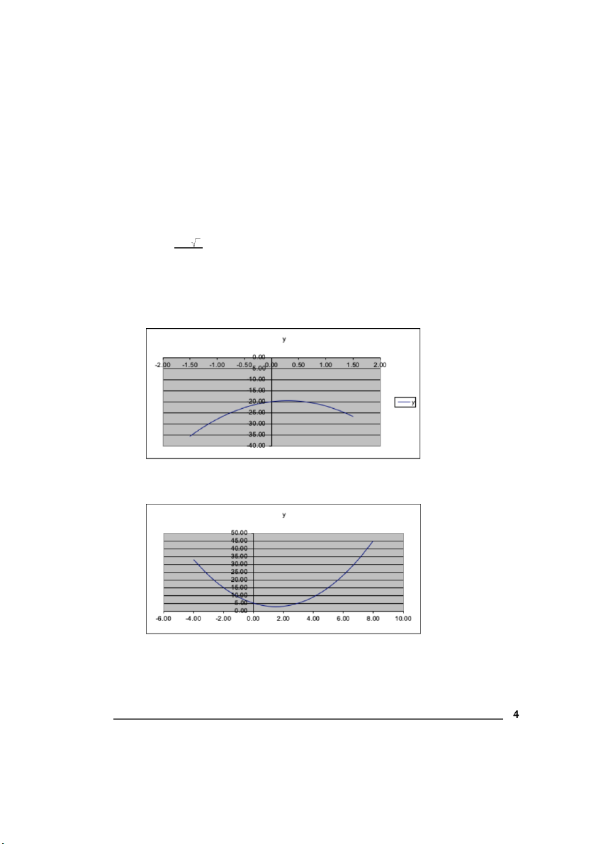
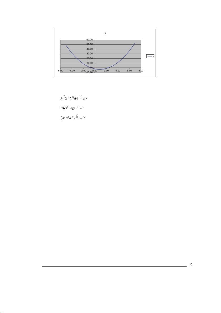
d. Equation 1:
Equation 2:
Equation 3:
8. Simplify the following mathematical functions:
Ans:
8 2 2 64
1/3 1/2 1/2 −1/2
= 2. 2 . (1/8) = 2. (2/8) = 0. 5
1/2
. 2
1/2
𝑙𝑛𝑒 𝑙𝑜𝑔10
5 5
= 5(1). 5(1) = 25
(𝑎 )
3
𝑎
3
𝑎
4
1/10
= (𝑎 )
10
1/10
= 𝑎
10/10
= 𝑎
9. Logarithms are usually to the base 10 or e, but this need not be the case. Find:
log
3
(9) = ?
log
4
(256) = ?
log
0.5
(0.125) = ?
Ans:
as
𝑙𝑜𝑔
3
(9) = 2 3
2
= 9
as
𝑙𝑜𝑔
4
(256) = 4 4
4
= 256
as
𝑙𝑜𝑔
0.5
(0. 125) = 3 0. 5 = 0. 125
3
10. Below is a table showing a series of numbers as well as their logarithms
1
and the changes in these
logarithms, with some numbers removed and marked with an X:
Number
Log
Change in Log
50.0
1.70
60.0
1.78
0.08
X
X
0.08
X
1.94
X
Please copy this table then fill in the missing numbers. What is the constant percentage change
between the numbers?
Ans:
1.2
Number
Log
Change in
Log
50.0
1.70
60.0
1.78
0.08
72.0
1.86
0.08
86.4
1.94
0.08
11. The general form of the exponential (or semi-log) function is written as:
𝑌
𝑡
= β
0
. 𝑒
β
1
𝑡
In its current form this is a nonlinear function and so cannot be estimated using linear regression.
Use logarithms to convert this function so that it can be estimated using linear regression. Once the
function has been estimated, what does β
1
represent?
Ans:
Use logarithms to convert this function so that it can be estimated using linear regression:
𝑌
𝑡
= β
0
. 𝑒
β
1
𝑡
=>
𝑙𝑛 𝑌 = 𝑙𝑛 (β
𝑡 0
. 𝑒 )
β
1
𝑡
1
Note that the logarithms have been rounded to two decimal places.
=>
𝑙𝑛 𝑌 = 𝑙𝑛 β 𝑙𝑛 𝑒
𝑡 0
+ β
1
𝑡
=> 𝑙𝑛 𝑌 = 𝑙𝑛 β
𝑡 0
+ β 𝑡
1
β
1
represent the growth rate per unit change in time
12. The following function relates the quantity of good Y sold (Q ) to its own price (P
y y
), the price of another
good X (P
x
) and income levels (INC).
Q P
y
= β
0 y
β1
.P
x
β2
.INC
β3
Again use logarithms to convert this function into a form that can be estimated using linear regression.
Once estimated, what do the values of represent? What does the sign ofβ
1
, β
2
and β
3
β
2
indicate?
Ans:
𝑄
𝑌
= β
0
𝑃
𝑌
β
1
𝑃
𝑋
β β
2
𝐼𝑁𝐶
3
𝑙𝑛 𝑄 = 𝑙𝑛 β + 𝑙𝑛 𝑃
𝑌 0 𝑌
β
1
+ 𝑙𝑛 𝑃
𝑋
β β
2
+ 𝑙𝑛 𝐼𝑁𝐶
3
𝑙𝑛 𝑄 = 𝑙𝑛 β 𝑙𝑛 𝑃 𝑙𝑛 𝑃 𝑙𝑛 𝐼𝑁𝐶
𝑌 0
+ β
1 𝑌
+ β
2 𝑋
+ β
3
β
1
: 𝑜𝑤𝑛 𝑝𝑟𝑖𝑐𝑒 𝑒𝑙𝑎𝑠𝑡𝑖𝑐𝑖𝑡𝑦 𝑜𝑓 𝑑𝑒𝑚𝑎𝑛𝑑
β
2
: 𝑐𝑟𝑜𝑠𝑠 𝑝𝑟𝑖𝑐𝑒 𝑒𝑙𝑎𝑠𝑡𝑖𝑐𝑖𝑡𝑦 𝑜𝑓 𝑑𝑒𝑚𝑎𝑛𝑑
β
3
: 𝑖𝑛𝑐𝑜𝑚𝑒 𝑒𝑙𝑎𝑠𝑡𝑖𝑐𝑖𝑡𝑦
If , substitutes.β
2
> 0 𝑋 𝑎𝑛𝑑 𝑌
If , complements.β
2
< 0 𝑋 𝑎𝑛𝑑 𝑌
| 1/7

Preview text:

QUANTITATIVE METHODS IN FINANCE TUTORIAL LECTURE 1 1.
What is the intercept, slope and elasticity for the following function: y = a + bx +cx2 Ans: the intercept = a
slope: 𝑑𝑦 = 𝑏 + 2𝑐𝑥 𝑑𝑥 𝑥 𝑥 the elasticity: 𝑑𝑦 = (𝑏 + 2𝑐𝑥) 𝑑𝑥 𝑦 𝑦 2.
If t (time) is the independent variable, what is the growth rate for this function: y = a + b.t + c.t2 Ans: 𝑑𝑦 1 growth rate 𝑑𝑦 = 𝑦 = 𝑑𝑡 𝑑𝑡 𝑦 𝑑𝑦 1 As: 𝑑𝑦 1 = 𝑏 + 2𝑐𝑡 nên = (𝑏 + 2𝑐𝑡) 𝑑𝑡 𝑑𝑡 𝑦 𝑦 3.
If t (time) is the independent variable, what is the growth rate for this function: y = eat Ans: 𝑑𝑦 1 the growth rate 𝑑𝑦 = 𝑦 = 𝑑𝑡 𝑑𝑡 𝑦 𝑑𝑦 𝑎𝑡 𝑑𝑦 1 𝑎𝑡 1 1 As:
= 𝑒 𝑎 , the growth rate is = 𝑒 𝑎 = 𝑦𝑎 = 𝑎 𝑑𝑡 𝑑𝑡 𝑦 𝑦 𝑦 4.
For the function y = xa, prove that the elasticity equals “a”. Ans: 𝑎 𝑦 = 𝑥 𝑑𝑦 𝑎−1 = 𝑎𝑥 𝑑𝑥 𝑎−1 𝑎 −1 𝑥 𝑦 => 𝑥 η = 𝑎𝑥 = 𝑎𝑥 𝑥 = 𝑎 = 𝑎 𝑦 𝑦 𝑦 5.
Suppose the price movements of an asset can be modeled as a continuous return. That is, p R t = pt-1.e .
Define R in terms of pt and pt-1. 6.
Using the following financial models as examples: ● write down their equations, ●
explain what type of equations they are, and ●
briefly describe the key properties of each type of equation. a.
The Market Model Characteristic Line. b.
The Capital Market Line (CML), part of the Capital Asset Pricing Model (CAPM). c.
The security market line (SML), also part of CAPM. d.
An equation used in the arbitrage pricing theory (APT) model. Ans:
The key features of these Linear Functions are as follows:
a. Securities Characteristic Line 𝑅 = β + β 𝑅 𝑖𝑡 0 1 𝑀𝑡 - Independent Variable: 𝑅𝑀 - Dependent variable : 𝑅𝑖 - Intercept: β = 𝑅 0 𝑓 - Slope: β1 b. Capital Market Line 𝐸(𝑅 )−𝑅 [ ]
𝐸(𝑅 ) = β + β 𝑆𝐷(𝑅 ) = 𝑅 + 𝑀 𝑓 𝑆𝐷(𝑅 ) 𝑃 0 1 𝑃 𝑓 𝑆𝐷(𝑅 ) 𝑃 𝑀 -
Independent variables : 𝑆𝐷(𝑅 ) 𝑃 -
Dependent variable: 𝐸(𝑅 ) 𝑃 - Intercept: 𝑅𝑓 𝐸(𝑅 )−𝑅 [ ] - Slope: 𝑀 𝑓 𝑆𝐷(𝑅 ) 𝑀 c. Security market line
𝐸(𝑅 ) = 𝑅 + 𝐸(𝑅 ) − 𝑅 [ ]β 𝑖 𝑓 𝑀 𝑓 𝑖 - Independent Variable: β𝑖 -
Dependent variable: 𝐸(𝑅 ) 𝑖 - Intercept: 𝑅𝑓 - Slope: 𝐸(𝑅 [ ) − 𝑅 ] 𝑀 𝑓 d. Arbitrage pricing theory
𝐸(𝑅 ) = 𝑅 + 𝐸(𝑅 ) − 𝑅 [ ]β + 𝐸(𝑅 ) − 𝑅 [ ]β 𝑖 𝑓 𝐹1 𝑓 𝑖,𝐹1 𝐹2 𝑓 𝑖,𝐹2 - Independent Variables: β , β the systematic risks, 𝑖,𝐹1 𝑖,𝐹2 -
Dependent variable: 𝐸(𝑅 ) 𝑖 - Intercept: 𝑅𝑓 - Slope: 𝐸(𝑅 [ ) − 𝑅 , ] 𝐸(𝑅 [ ) − 𝑅 ] 𝐹1 𝑓 𝐹2 𝑓 7. For the following functions: 2 0 =− 5𝑥 + 3𝑥 − 20 2 0 = 𝑥 − 2. 5𝑥 − 2. 5 2 0 = 1. 5𝑥 − 3𝑥 + 5 a.
What are their discriminations? b.
What is the significance of these discriminations? c.
Complete the square and thereby solve for x for these equations (please do this both by hand and using the
excel solver, see excel instructions below). d.
Use excel to graph these functions. To use the solver: 2 ➢
construct the formula for the equation 0 =− 5𝑥 + 3𝑥 − ; 20 in B1: SUM(C1: E1), C1:
=-5*C2^2, D1: = 3*C2, E1: = -20, C2: the starting value for x. ➢
go to solver (tools or formula), Set Cell $B$1, Equal To 0, By Changing C2, Solve. ➢
keep trying different starting values of x until you have found all solutions. ➢
if you have trouble go to help. Ans: a. Function 1: 2 2
∆ = 𝑏 − 4𝑎𝑐 = 3 − 4(− 5)(− 20) = − 391 1 Function 2: 2 2
∆ = 𝑏 − 4𝑎𝑐 = (− 3) − 4(1)(5) = − 11 2 Function 3: 2 2
∆ = 𝑏 − 4𝑎𝑐 = (− 2. 5) − 4(1. 5)(− 2. 5) = 21. 25 3 2
b. The formula 𝑏 − 4𝑎𝑐 known as the discriminant. 2
If 𝑏 − 4𝑎𝑐 > 0, there are two values of x that satisfy the equation 2
If 𝑏 − 4𝑎𝑐 = 0, there is one value of x that satisfy the equation 2
If 𝑏 − 4𝑎𝑐 < 0, there are no values of x that satisfy the equation.
The discriminant part of the formula is used for finding the roots of a quadratic equation. That is, 2
finding the value(s) of x that satisfy this equation: 0 = 𝑎𝑥 + 𝑏𝑥 + 𝑐
c. Both equations 1 and 2 have no values of x that satisfy these equations . Equation 3 has 2 values of x: −𝑏± ∆ 𝑥 = 1,2 2𝑎 𝑥 = 2. 37 1 𝑥 = − 0. 70 2 d. Equation 1: Equation 2: Equation 3: 8.
Simplify the following mathematical functions: Ans: 1/3 1/2 1/2 −1/2 1/2 1/2 8 2 2 64 = 2. 2 . 2 . (1/8) = 2. (2/8) = 0. 5 5 5
𝑙𝑛𝑒 𝑙𝑜𝑔10 = 5(1). 5(1) = 25 1/10 1/10 3 3 4 10 10/10 (𝑎 𝑎 𝑎 ) = (𝑎 ) = 𝑎 = 𝑎 9.
Logarithms are usually to the base 10 or e, but this need not be the case. Find: log 3(9) = ? log 4(256) = ? log 0.5(0.125) = ? Ans: 2 𝑙𝑜𝑔 (9) = 2 as 3 = 9 3 4
𝑙𝑜𝑔 (256) = 4 as 4 = 256 4 3
𝑙𝑜𝑔 (0. 125) = 3 as 0. 5 = 0. 125 0.5
10. Below is a table showing a series of numbers as well as their logarithms1 and the changes in these
logarithms, with some numbers removed and marked with an X: Number Log Change in Log 50.0 1.70 60.0 1.78 0.08 X X 0.08 X 1.94 X
Please copy this table then fill in the missing numbers.
What is the constant percentage change between the numbers? Ans: Change in 1.2 Number Log Log 50.0 1.70 60.0 1.78 0.08 72.0 1.86 0.08 86.4 1.94 0.08
11. The general form of the exponential (or semi-log) function is written as: β 𝑡 𝑌 = β . 𝑒 1 𝑡 0
In its current form this is a nonlinear function and so cannot be estimated using linear regression.
Use logarithms to convert this function so that it can be estimated using linear regression. Once the
function has been estimated, what does β1 represent? Ans:
Use logarithms to convert this function so that it can be estimated using linear regression: β 𝑡 𝑌 = β . 𝑒 1 𝑡 0 β 𝑡
=> 𝑙𝑛 𝑌 = 𝑙𝑛 (β . 𝑒 1 ) 𝑡 0
1 Note that the logarithms have been rounded to two decimal places. 𝑡
=> 𝑙𝑛 𝑌 = 𝑙𝑛 β + β 𝑙𝑛 𝑒 𝑡 0 1
=> 𝑙𝑛 𝑌 = 𝑙𝑛 β + β 𝑡 𝑡 0 1
β1 represent the growth rate per unit change in time
12. The following function relates the quantity of good Y sold (Qy) to its own price (Py), the price of another
good X (Px) and income levels (INC). Q β1 β2 y = β0Py .Px .INC β3
Again use logarithms to convert this function into a form that can be estimated using linear regression.
Once estimated, what do the values of β1, β2 and β3 represent? What does the sign of β2 indicate? Ans: β β β
𝑄 = β 𝑃 1𝑃 2𝐼𝑁𝐶 3 𝑌 0 𝑌 𝑋 β β β
𝑙𝑛 𝑄 = 𝑙𝑛 β + 𝑙𝑛 𝑃 1 + 𝑙𝑛 𝑃 2 + 𝑙𝑛 𝐼𝑁𝐶 3 𝑌 0 𝑌 𝑋
𝑙𝑛 𝑄 = 𝑙𝑛 β + β 𝑙𝑛 𝑃 + β 𝑙𝑛 𝑃 + β 𝑙𝑛 𝐼𝑁𝐶 𝑌 0 1 𝑌 2 𝑋 3
β : 𝑜𝑤𝑛 𝑝𝑟𝑖𝑐𝑒 𝑒𝑙𝑎𝑠𝑡𝑖𝑐𝑖𝑡𝑦 𝑜𝑓 𝑑𝑒𝑚𝑎𝑛𝑑 1
β : 𝑐𝑟𝑜𝑠𝑠 𝑝𝑟𝑖𝑐𝑒 𝑒𝑙𝑎𝑠𝑡𝑖𝑐𝑖𝑡𝑦 𝑜𝑓 𝑑𝑒𝑚𝑎𝑛𝑑 2
β : 𝑖𝑛𝑐𝑜𝑚𝑒 𝑒𝑙𝑎𝑠𝑡𝑖𝑐𝑖𝑡𝑦 3 If β > ,
0 𝑋 𝑎𝑛𝑑 𝑌 substitutes. 2
If β < 0, 𝑋 𝑎𝑛𝑑 𝑌 complements. 2