Bài 7.1: Lý thuyết cơ sở của BT giá trị ban đầu trong Phương trình Vi phân. Môn Phương pháp tính trong kỹ thuật (UET) | Trường Đại học Công nghệ, Đại học Quốc gia Hà Nội.

lOMoAR cPSD| 58833082
Bài 7.1 Lý thuyết cơ sở của BT giá trị ban đầu
Differential equations are used to model problems in science
and engineering that involve the change of some variable with
respect to another. Most of these
problems require the solution of
an initial-value problem, that is,
the solution to a differential 1 lOMoAR cPSD| 58833082
equation that satisfies a given initial condition.
In common real-life situations,
the differential equation that models the problem is too complicated to solve exactly, and one of two approaches is taken to approximate the solution.
The first approach is to modify
the problem by simplifying the
differential equation to one that
can be solved exactly and then 2 lOMoAR cPSD| 58833082 use the solution of the simplified equation to approximate the solution to the original problem. The other approach, which we will examine in this chapter, uses methods for approximating the solution of
the original problem. This is the approach that is most commonly taken because the approximation methods give more 3 lOMoAR cPSD| 58833082
accurate results and realistic error information. The methods that we consider
in this chapter do not produce a
continuous approximation to the solution of the initial-value problem. Rather, approximations are found at certain specified, and often equally spaced, points. Some method of interpolation, commonly Hermite, is used if
intermediate values are needed. 4 lOMoAR cPSD| 58833082 We need some definitions and results from the theory of
ordinary differential equations
before considering methods for
approximating the solutions to initial-value problem
Definition 7.1 A function f (t, y)
is said to satisfy a Lipschitz
condition in the variable y on a
set D R2 if a constant L > 0 exists with
|f (t, y1) - f (t, y2, )| ≤ L| y1 - y2|,
whenever (t, y1) and (t, y2) are 5 lOMoAR cPSD| 58833082
in D. The constant L is called a
Lipschitz constant for f
Example 1 Show that f (t, y) = t|
y| satisfies a Lipschitz condition
on the interval D = {(t, y) | 1 ≤ t
≤ 2 and - 3 ≤ y ≤ 4}.
Solution For each pair of points
(t, y1) and (t, y2) in D we have
|f (t, y1) - f (t, y2)| = |t| y1| - t|
y2||= |t| y1| - | y2 ≤ 2| y1 - y2|.
Thus f satisfies a Lipschitz
condition on D in the variable y
with Lipschitz constant 2. The 6 lOMoAR cPSD| 58833082
smallest value possible for the Lipschitz constant for this
problem is L = 2, because, for example,
|f (2, 1) - f (2, 0)| = |2 - 0| = 2|1 - 0|.
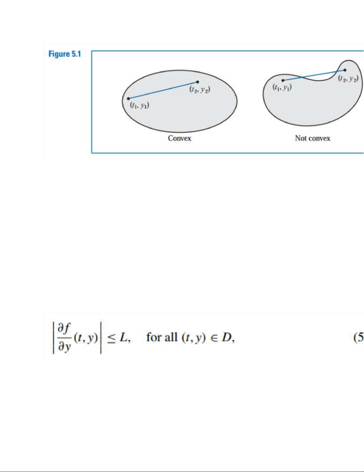
Definition 7.2 A set D R2 is
said to be convex if whenever
(t1, y1) and (t2, y2) belong to D, then
((1 - λ)t1 + λt2, (1 - λ)y1 + λy2)
also belongs to D for every λ in [0, 1]. 7 lOMoAR cPSD| 58833082
In geometric terms, Definition
5.2 states that a set is convex provided that whenever two points belong to the set, the entire straight-line segment
between the points also belongs
to the set. (See Figure 5.1.) The
sets we consider in this chapter
are generally of the form D =
{(t, y) | a ≤ t ≤ b and -∞ < y <
∞} for some constants a and b. It is easy to verify 8 lOMoAR cPSD| 58833082
(see Exercise 7) that these sets are convex. 9 lOMoAR cPSD| 58833082
Theorem 7.3 Suppose f (t, y) is
defined on a convex set D ⊂
R2. If a constant L > 0 exists with
for all (t, y) ∈ D, (5.1) then f
satisfies a Lipschitz condition 10 lOMoAR cPSD| 58833082
on D in the variable y with Lipschitz constant L. The proof of Theorem 7.3 is
discussed in Exercise 6; it is similar to the proof of the corresponding result for functions of one variable discussed in Exercise 27 of Section 1.1.
As the next theorem will show,
it is often of significant interest 11 lOMoAR cPSD| 58833082 to determine whether the
function involved in an initial- value problem satisfies a Lipschitz condition in its
second variable, and condition (5.1) is generally easier to apply than the definition. We should note, however, that Theorem 5.3 gives only sufficient conditions for a Lipschitz condition to hold. The function in Example 1, for instance, 12 lOMoAR cPSD| 58833082
satisfies a Lipschitz condition, but the
partial derivative with respect to
y does not exist when y = 0. The following theorem is a version of the fundamental existence and uniqueness
theorem for first-order ordinary
differential equations. Although
the theorem can be proved with the hypothesis reduced somewhat, this form of the theorem is sufficient for our 13 lOMoAR cPSD| 58833082 purposes. (The proof of the
theorem, in approximately this form, can be found in [BiR], pp. 142–155.)
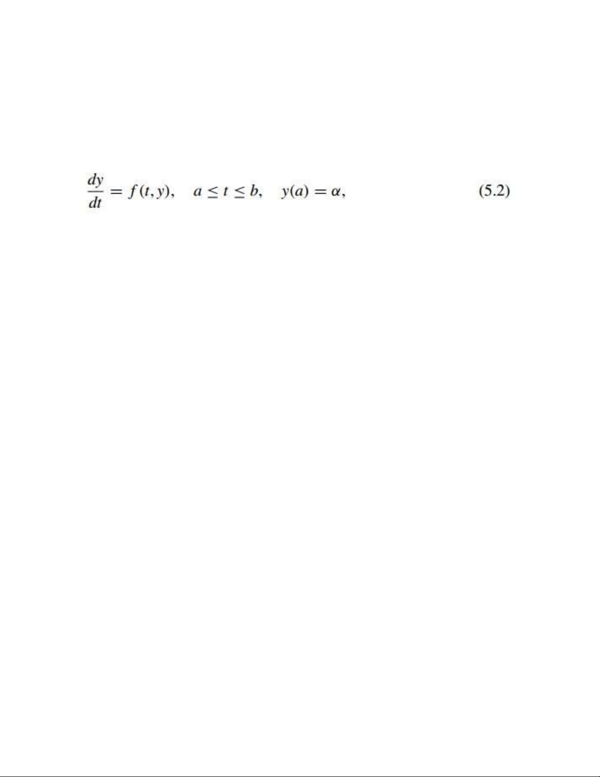
Theorem 7.4 Suppose that D =
{(t, y) | a ≤ t ≤ b and -∞ < y <
∞} and that f (t, y) is continuous
on D. If f satisfies a Lipschitz
condition on D in the variable y,
then the initial-value problem
y’(t) = f (t, y), a ≤ t ≤ b, y(a) =
α, has a unique solution y(t) for
a ≤ t ≤ b. 14 lOMoAR cPSD| 58833082
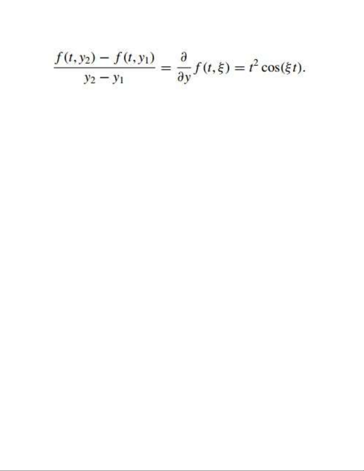
Example 2 Use Theorem 5.4 to show that there is a unique solution to the initial-value problem
y’ = 1 + t sin(ty), 0 ≤ t ≤ 2, y(0) = 0.
Solution Holding t constant and applying the Mean Value
Theorem to the function f (t, y)
= 1 + t sin(ty), we find that
when y1 < y2, a number ξ in
(y1, y2) exists with 15 lOMoAR cPSD| 58833082 Thus
|f (t, y2) - f (t, y1)| = | y2 - y1||t2
cos(ξt)| ≤ 4|y2 - y1|,
and f satisfies a Lipschitz
condition in the variable y with
Lipschitz constant L = 4.
Additionally, f (t, y) is
continuous when 0 ≤ t ≤ 2 and
∞ < y < ∞, so Theorem 5.4
implies that a unique solution 16 lOMoAR cPSD| 58833082 exists to this initial-value problem.
If you have completed a course in differential equations you might try to find the exact solution to this problem. Well-Posed Problems Now that we have, to some extent, taken care of the
question of when initial-value
problems have unique solutions, we can move to the second
important consideration when 17 lOMoAR cPSD| 58833082
approximating the solution to an initial-value problem.
Initialvalue problems obtained by observing physical phenomena generally only
approximate the true situation, so we need to know whether
small changes in the statement of the problem introduce correspondingly small changes in the solution. This is also important because of the
introduction of round-off error 18 lOMoAR cPSD| 58833082 when numerical methods are used. That is, • Question: How do we
determine whether a particular problem has the property that
small changes, or perturbations,
in the statement of the problem introduce correspondingly
small changes in the solution?
As usual, we first need to give a
workable definition to express this concept. 19 lOMoAR cPSD| 58833082
Definition 5.5 The initial-value problem
is said to be a well-posed problem if:
• A unique solution, y(t), to the problem exists, and
• There exist constants ε0 > 0
and k > 0 such that for any ε,
with ε0 > ε > 0, whenever δ(t)
is continuous with |δ(t)| < ε for 20