Bài báo cáo cuối kỳ môn Tính toán động cơ đốt trong đề tài "Project Mazda 6" bằng tiếng Anh

lOMoARcPSD| 36991220
Ho Chi Minh City University of
Technology and Education
Faculty of Vehicle and Energy Engineering
Department of Internal Combustion Engine PROJECT MAZDA 6
Subject: INTERNAL COMBUSTION ENGINE CALCULATION lOMoARcPSD| 36991220 Contents
1. Engine parameters...........................................................................................5 2. Report
content..................................................................................................5 3.
Curves.............................................................................................................5
CHAPTER 1: THERMAL CALCULATE.................................................6
2.1 Parameters of Mazda 6........................................................................................6
2.2 Choose parameter for thermal calculate.............................................................6
2. 1.1 Intake Air Pressure (P0)...................................................................................6 2.2. 2 Intake Air Temperature
(T0)............................................................................7 2.3.3
The Compressor Outlet Air Pressure (Pk)........................................................7 2.4.4
The Compressor Outlet Air Temperature (Tk).................................................7 2.5.5
Pressure At The End Of Intake (Pa).................................................................7 2.6.6
Pressure Of Sesidual Gases (Pr)......................................................................7 2.7.7
Temperature Of Sesidual Gases (Tr)................................................................7 2.8.8
Fresh Charge Preheating Temperature (∆T)....................................................8 2.2.9
1 Factor..........................................................................................................8 2.2.10
2 Factor........................................................................................................8 2.2.11
t Factor.........................................................................................................8 2.2.12
Heat gain coefficient at point Z ξz.................................................................9 2.2.13
Heat gain coefficient at point B ξb................................................................9 2.2.14
ir residue coefficient α................................................................................9 2.2.15
Choose the coefficient to fill the work graph 𝝋d...........................................9 2.3.2.4
The compression means polytropic index n1..............................................................11 1 2.2.16
Turbo ratio.....................................................................................................9
2.3 Thermal calculate.................................................................................................10 2 2.3.1
Intake Process..............................................................................................10 3 2.3.1.1
Volumetric effciency (ηv)................................................................10 4 2.3.1.2
Coefficient of residual gases (𝝋ᵣ).....................................................10 2.3.1.3
Temperature at the end of induction (Ta).................................................................10 5 2.3.2
Compress Process........................................................................................10 6 2.3.2.1
The mean molar specific heat of the air..........................................10
7 2.3.2.2The mean molar specific heat of residual gases at the the end of
compression.....................................................................................................11
8 2.3.2.3The mean molar specific heat of the working mixture.........................11 lOMoARcPSD| 36991220 2.3. 9.5
The pressure at the end of compression process..................................11 2.3.10.6
The temperature at the end of compression process (Tc).....................11 11.3.3
Combustion Process......................................................................................12 12.3.3.1
Theoretical air requirement in kmoles needed for the combustion of 1
kg of fuel (M0)................................................................................................12
2.3.3. 13 The actual quantity of air participating in combustion of 1 kg of fuel (M1) 12 14.3.3.3
The tottal amount of combustion products (M2)..................................12 15.3.3.4
The theory molecular change coefficient of combustible mixture (β0)13 16.3.3.5
The actual molecular change coefficient of combustible mixture (β) .13 17.3.3.6
The molecular change coefficient of combustible mixture points Z (βZ)
..........................................................................................................................13 2.3.3.7
Chemically incomplete combustion of
fuel.........................................13 2.3.3.8
The molar specific heat of the working mixture at point Z.................13 2.3.3.9
The temperature at the end of combustion
process..............................14 2.3.3.10
The pressure at the end of combustion
process.................................14 2.3.4. Expand
procces.............................................................................................14 2.3.4.1
Preexpansion in the case of heat added at constant pressure( ρ).........14 2.3.4.2
After expansion (ε)..............................................................................14 2.3.4.3
The expansion mean polytropic index (n2)..........................................14 2.3.4.4
The temperature at the end of expansion process................................15 2.3.4.5
The pressure at the end of expansion process......................................15
9 2.4.1Calculated average indicated pressure pi'..................................................15
10 2.4.2Actual average indicated pressure.............................................................15
11 .4.3 Mechanical loss pressure...........................................................................16
2.4.4 Mean effective pressure............................................................................16
12 2.4.5Mechanical efficiency...............................................................................16
13 2.4.6Indicator efficiency...................................................................................16
14 2.4.7Effective (thermal) efficiency...................................................................16
15 2.4.8The indicator specific fuel consumption...................................................16
16 2.4.9The effective specific fuel consumption....................................................16
17 2.4.10Cylinder-size effects...............................................................................16 lOMoARcPSD| 36991220 2.3.4.6
Test for temperature of residual gases.................................................15 2.3.4.7
Error of residual gases.........................................................................15
2.4. Calculate typical parameters of the
cycle.........................................................15
3. Curves................................................................................................................1 9 lOMoARcPSD| 36991220
CHAPTER 2: CALCULATION OF PISTON DYNAMICS AND
CRANKSHAFT - CONDUCTING ROD STRUCTURE DYNAMICS .20 I.
Kinetics of the piston....................................................................................20 1.
Piston displacement...............................................................................20 2.
Piston speed...........................................................................................21 3.
Piston acceleration.................................................................................22
II. Dynamics of the crankshaft - connecting rod mechanism.........................23
1.Pneumatic force..........................................................................................23
2.Inertial force of moving parts.....................................................................24 lOMoARcPSD| 36991220 1. Engine parameters Engine: Skyactiv G2.5 Stroke, : 4 Nemax (kW): 100 RPM: 6000 Compression ratio, : 13:1 Air equivalence ratio ( ): 0,9 Cooling system: Air&Water No of cylinder, i: 4
Angle of open(close) intake(exhaust) valve Open Close Intake valve 15o BTDC 45o ABDC Exhaust valve 40o BBDC 100 ATDC 2. Report content
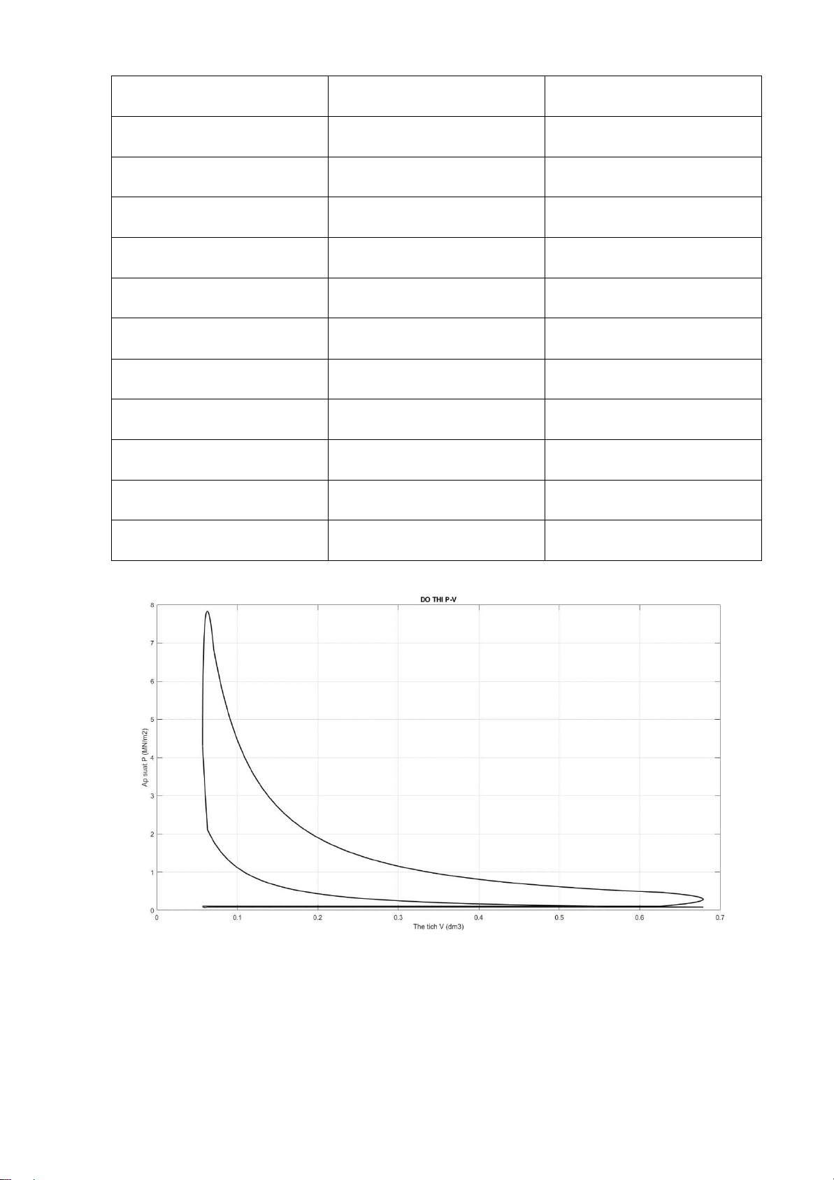
2.1 Thermal calculate and buid indicated work diagram in engine.
2.2 Kinetic and dynamic of slider crank mechanism. 3. Curves 3.1 P – V figure 3.2 P – , PJ, P1 figures
3.3 Kinetic and dynamic figures
Deadline: week 15 ............................................................... Advisor lecturer (Sign and full name) Associate Prof. Ly Vinh Dat
CHAPTER 1: THERMAL CALCULATE
2.1 Parameters of Mazda 6 No. Name Symbol Value Unit Note lOMoARcPSD| 36991220 1. Engine type Gasoline engine 2. Stroke 4 3. Displacement stroke S 100 mm 4. Number of cylinder i 4 5. Bore diameter B 89 mm STD 6. Piston weight mnp 133.6 kg/m^2 7. Conecting rod lenght L 154,8 mm STD 8. Conecting rod weight mcr 178 kg/m^2 9. Max power Nemax 100 kW 6000rpm 10. Max torque Tmax 185 Lb-ft 3250rpm 11. Compress ratio 𝝋 13:1 12. Fuel supply GDI 13. Coolant system Air & Liquid 14. Structural parameter S/D 1,12 =R/L 0,30
2.2 Choose parameter for thermal calculate 2.2.1
Intake Air Pressure (P0)
Intake air pressure is a barometric pressure, value of P0 is depends on
altitude of sea level. If altitude increase, P0 will decrease becase the air becomes
thinner.At altitude of sea level: P0=0,1013 MN/m2 2.2.2
Intake Air Temperature (T0)
Intake air temperature depends on average temperature where the vehicle
operated.It’s difficult for vehicle designed to operated where the range of
temperature variation during the day is large.
South Viet Nam is belonging tropic region so average temperature during
the day is tkk=29oC for South Viet Nam, then: lOMoARcPSD| 36991220 T0 = Tkk + 273=302 oK 2.2.3
The Compressor Outlet Air Pressure (Pk)
Non-Turbocharge 4-Stroke engine: Pk = P0 = 0,1013 MN/m2 2.2.4
The Compressor Outlet Air Temperature (Tk)
Non-Turbocharge 4-Stroke engine: Tk = T0 = 302 oK 2.2.5
Pressure At The End Of Intake (Pa)
Intake air pressure at the end of intake stroke is always smaller than intake
pressure before coming through intake valve because volume loss in intake manifold and throttle.
With Non-turbocharge 4-Stroke engine Pa = (0,80÷ 0,95)P0.
Choose value efficiency = 0,8: Pa= 0,08104 MN/m2 2.2.6
Pressure Of Sesidual Gases (Pr)
With gasoline engine, air pressure extant after exhaust stroke, Pr = (0,11÷0,12) MPa Choose P r= 0,11 Mpa 2.2.7
Temperature Of Sesidual Gases (Tr)
In ICEC, usually take Tr at the end of exhaust stroke.
Value of Tr depends on many factor as compress ratio 𝝋, air equivalence ( ), speed of crankshaft,
Value of 𝝋 high then mixtur burning more expands so Tr is small.
In gasoline engine, value of Tr = (900÷1000)oK Take Tr = 970 oK lOMoARcPSD| 36991220 2.2.8
Fresh Charge Preheating Temperature (∆T)
During the cylinder filling process, the temperature of a fresh charge
somewhat increases due to hot parts of the engine. The value of preheating ∆T is
dependent on the arrangement and construction of the intake manifold, cooling
system, use of a special preheater, engine speed and supercharging. Increased
temperature improves fuel evaporation, but decreases the charge density, thus
affecting the engine volumetric efficiency. These two factors in opposition
resulting from an increase in the reheating temperature must be taken into
account in defining the value of ∆T.
In gasoline engine, ∆T = (0÷20)oC Take ∆T = 20oC 2.2.9 1 Factor Take 1 = 1,05 2.2.10 2 Factor Take 2 = 1 2.2.11 t Factor
t factor depends on Air equivalence ratio and Air Temperature After
Exhaust Stroke, according to experiments with gasoline engine, t is take: Air equivalence ratio ( )
Specific heat correction factor ake t = 1,15 2.2.12
Heat gain coefficient at point Z ξz Take z = 0,80 2.2.13
Heat gain coefficient at point B ξb lOMoARcPSD| 36991220 Take b = 0,86 2.2.14
ir residue coefficient α
The coefficient α greatly affects the combustion process: For internal
combustion engines, calculation.
The heat usually has to be calculated in maximum power mode, the air residue
coefficient is selected in the range is given in the following table: Engine types α Gasoline 0.85 ÷ 0.95 Choose α = 0.85. 2.2.15
Choose the coefficient to fill the work graph 𝝋d Take 𝝋d = 0,93 2.2.16 Turbo ratio
It is the ratio between the pressure of the gas mixture in the cylinder at the
end of combustion and too compressor.
The λ value is usually in the following range:
Gasoline engine: λ = 3.00 ÷ 4.00 Take λ = 3.00 2.3 Thermal calculate. 2.3.1 Intake Process 2.3.1.1
Volumetric effciency (ηv) η = 1 . 1 Tₖ Pₐ − 𝝋ᵣ 𝝋 lOMoARcPSD| 36991220 18 ε-1 (T +∆Tₖ ) Pₖ 1 𝝋 2 (𝝋ₐ) ]
With m is average multivariate expand index of air extant after exhaust stroke. Take m = 1.45 1 ηv= 1 . 302
.0,08104 . [13.1,02 − 1,15.1. ( 0,11 )1,45] 13-1 (302+20) 0,1013 0,08104 ηv=0,74 2.3.1.2
Coefficient of residual gases (𝝋ᵣ) γ = ₂. . Pᵣ . Tₖ = 1 0,11 . 302 =0,038 r . (ε-1).ηᵥ P ₖ Tᵣ (13-1).0,74 0,1013 970 2.3.1.3
Temperature at the end of induction (Ta) 𝝋 − 1
(Tₖ+ ∆T) + (𝝋ᵣ𝝋ₐ) ( 𝝋 ) Ta= ₜ ᵣ.γ .T .ᵣ
(302+ 20) + 1,15.0,038.9701+. γᵣ(0,08104)(1,45 − 1,451) 0,11 = 1+0,038 Ta = 347,35(oK) 2.3.2 Compress Process 2.3.2.1
The mean molar specific heat of the air bv 0,00419 mc= aᵥ+ .T = 19,806 + .T
18 2 2 aᵥ=19,806 ; bv = 0,00419 lOMoARcPSD| 36991220 2.3.2.19
The mean molar specific heat of residual gases at the the end of compression. m̅
c̅ᵥ"= (17,997+3,504α) + 1 ( 360,34+ 184,36) .10-5.T 2 α Where α=0,85
𝝋′′𝝋 = 20,98; 𝝋′′𝝋 = 2,87. 10−3 2.3.20.3
The mean molar specific heat of the working mixture. m̅
cᵥ̅'= mcᵥ + γᵣ.mcᵥ " =a' + bv' .T v 1+ γᵣ 2
19.806 + 2,095.10−3.T+ 0,038.(20,98+2,87.10−3. T) 1+ 0,038 = a' +v b2v' .T
𝝋′𝝋 = 19,85; 𝝋′𝝋 = 2,12.10−3 2.3.2.4
The compression means polytropic index n1 8.314 = 8.314 n₁-1= bᵥ' 1
19,85+2,21.10−3.347,35.(13n1-1+1)
19 .3.2.5 The pressure at the end of compression
process Pc= Pa.εn₁ =0,08104.131,37 = 2,72 (𝝋𝝋𝝋)
20 .3.2.6 The temperature at the end of compression process (Tc)
Tc= Ta. εn₁-1=347,35.131,37-1 = 897,27(oK) lOMoARcPSD| 36991220 aᵥ'+ 2 .Tₐ.(εn -1+1) 𝝋1 = 1,37 2.3.3 Combustion Process
2.3.3.1 Theoretical air requirement in kmoles needed for the combustion of 1 kg of fuel (M0)
Ingredients per 1 kg fuel (kg) Type of Content (kg) Molar mass QH (KJ/kg) fuel (kg/kmol) C H O Gasoline 0,855 0,145 --- 110-120 43960 1 C H O
M0= 0.21 . (12 + 4 - 32 ) = ⋯ (kmol. kk)
- Theoretical amount of air to burn 1kg of green: M0 = 0.516 kmol kk
2.3.3.2 The actual quantity of air participating in combustion of 1 kg of fuel (M1) 1 1 M = α.M₀ + = 0,85.0.516 + = 0,448 (kmol kk/kg.nl) 1 μ .lₙ 110
μ .ₙ 𝝋 is molar mass of gasoline; μ .ₙ 𝝋 = 110÷114 kg/kmol.
Choose μ .ₙ 𝝋 = 110 kg/kmol 2.3.3.3
The tottal amount of combustion products (M2) C H 0,855 0,145 M 2= 12 + 2 +0.79.α.M₀ = 12 + 2 + 0.79.0,85.0,516 𝝋𝝋𝝋 lOMoARcPSD| 36991220 = 0,49 (𝝋𝝋𝝋𝝋 𝝋𝝋) 𝝋𝝋
21.3.3.4 The theory molecular change coefficient of combustible mixture (β0) β = 0 M₂ = 0,49
= 35 (𝝋𝝋𝝋𝝋 𝝋𝝋𝝋 𝝋𝝋) M₁ 0,448 32 𝝋𝝋 222324.3.3.5
The actual molecular change coefficient of combustible mixture (β) 21 2.3.3.7
Chemically incomplete combustion of fuel
In engines operating at 𝝋 <1, we have chemically incomplete combustion of
fuel (J/lkg) because of lack of oxygen.
∆QH= 120.103.(1- 𝝋).M0 = 120.103.(1- 0,85).0,516= 9288 (KJ/kg.nl)
22 .3.3.8 The molar specific heat of the working mixture at point Z M₂
( 𝝋 + γᵣ) .mcᵥ' + M (1 − 𝝋) . mcᵥ mcv̅z′′ = 𝝋 β₀ 1𝝋 = a''vz +
𝝋 + γβ₀ᵣ ) + 𝝋₁ (1 − 𝝋)𝝋 𝝋₂ ( 𝝋 b''vz 0,75 0,038 0,75 2 .T 0,49. ( + ) .mcᵥ' + 0,448 (1 − ) . mcᵥ b'' 23 0,85 1,09 0,88 = a''
24 0,49. (00,,7585 + 0,0381,09 ) + 0,448. (1 − 00,,7585) vz + 2vz .T a''vz=19,84 b''vz= lOMoARcPSD| 36991220
In the cylinder of an actual engine a fuel-air mixture comprised by a fresh charge
(combustible mixture) M1 and residual gases then β=1+ β 1₀- =1+ 3235 -1 1+γᵣ 1+0,038
25.3.3.6 The molecular change coefficient of combustible mixture points Z (βZ) β₀-1 β =1+ 35 0,75 . 𝝋=1+ 32 -1 . = 1,08 Z 1+γᵣ 𝝋 1+0,038 0,85 2.3.3.9
The temperature at the end of combustion process
z𝝋(𝝋1(𝝋 1 + 𝝋 − ∆𝝋 ̅
𝝋)𝝋) + β̅zmc̅ᵥ̅'̅. Tc = . m̅ cᵥ′′. T𝝋 0,75. (44000 − 9288) =
+ (19,85 + 2,12. 10−3 . 𝝋 ). 𝝋 0,448. (1 + 0,038) 𝝋 𝝋
= 1,08. (19,84 + 2,1. 10−3. . 𝝋𝝋). 𝝋𝝋 T𝝋=2896,7310( K)⁰ 2.3.3.10
The pressure at the end of combustion process TZ
P𝝋 = βz TC . Pc = 1,08 897,27 . 2,72 P𝝋=8,95 (MPa) 25 ,1.10−3 lOMoARcPSD| 36991220 2.3.4 Expand procces 2.3.4.1
Preexpansion in the case of heat added at constant pressure( ρ) ρ=1 2.3.4.2
After expansion (ε) ε= 13 2.3.4.3
The expansion mean polytropic index (n2) ( b − z)QH β.m= ̅̅m̅̅̅ 8,314 T -βT ) ''.T -β ''.T + (β M1(1+γr) vb b z vz z n2-1 z z b n2-1 = ( b − z) Q H + 8,314 a'' + b'' vz .(T +T ) M1(1+γr).β(Tz-Tb) vz 2 z b Tz With T = and a'' =19,84 ; b'' = 2,1.10−3 b ε(n2-1) vz vz n2=1,23  2.3.4.4
The temperature at the end of expansion process 𝝋𝝋 𝝋𝝋 2733,03 = 𝝋𝝋2−1= 26 1,23−1 = 1515,09(⁰K) 26 3-1 1,23-1 13 1,37-1 13 = 1,07(𝝋𝝋𝝋) lOMoARcPSD| 36991220 27.3.4.5
The pressure at the end of expansion process With gasoline engine:
𝝋𝝋 = 𝝋𝝋𝝋𝝋2 = 138,195,23 = 0,38 (𝝋𝝋𝝋) 2.3.4.6
Test for temperature of residual gases 𝝋𝝋 𝝋−1𝝋 0,11 1,45−11,45 𝝋𝝋 = 𝝋𝝋 . (𝝋 𝝋 ) = 1515,09, . (0,38 ) = 1031,22(° 𝝋) 2.3.4.7
Error of residual gases |𝝋𝝋 − 𝝋𝝋𝝋|
𝝋𝝋 = 0,059 = 5,9% < 10%
2.4 Calculate typical parameters of the cycle 2.4.1
Calculated average indicated pressure (p'i) Pc p'= [ (ρ-1) + ρ. .β. (1- 1 ) - 1 (1- 1 )] i ε-1 𝝋 n2-1 δn2-1 n1-1 εn1-1
Replace ρ=1; δ=ε and 𝝋 = PPz then we have theoretical mean indicated c
pressure with heat added at constant volume (v=const) for gasoline engine Pc p p'= [ . (1- 1 ) - 1 (1- 1 )] 27 2.4.2
Actual average indicated pressure. lOMoARcPSD| 36991220 i ε-1 n2-1 εn2-1 n1-1 εn1-1 =[ 2,72 3,29 . (1- 1,23-11) - 1 . (1- 1,37-11)]
pi=φd.p'=0i,97.1,07=1,04 (MPa) lOMoARcPSD| 36991220 2.4.3
Mechanical loss pressure 𝝋.𝝋 100.6000.10−3 pV = 30 = 30= 20(m/s)
Pm = 𝝋 + 𝝋. Vp + (pr − pa) = 0,048 + 0,01512. 20 + (0,11 − 0,08104) = 0,38 (MPa) 2.4.4
Mean effective pressure.
pe=pi-pm=1,04-0,38=0,66 (MN/𝝋2) 2.4.5 Mechanical efficiency. ηe pe pm 0,38 η = = =1- = 1 − = 0,63 M ηi pi pi 1,04 2.4.6 Indicator efficiency.
𝝋𝝋 = 8,314. 𝝋1. 𝝋𝝋. 𝝋𝝋 = 8,314. 0,448 .1,04. 302 = 0,35 𝝋𝝋. 𝝋𝝋. 𝝋𝝋 44000 . 0,1013 . 0,74 2.4.7
Effective (thermal) efficiency
𝝋𝝋 = 8,314. 𝝋1. 𝝋𝝋. 𝝋𝝋 = 8,314. 0,46989 .0,80. 302 = 0,25 𝝋𝝋. 𝝋𝝋. 𝝋𝝋 43960 . 0,1013 .0,86 2.4.8
The indicator specific fuel consumption 3600 3600 g = i = = 0,23 Kg /kW. h H i lOMoARcPSD| 36991220 2.4.9
The effective specific fuel consumption 3600 3600 g = e = = 0,36kg /kW. h H 2.4.10 Cylinder-size effects
The engine displacement volume in litres is determined by the effective, power,
engine speed and effective pressure: 30. 𝝋. Ne 30.4.90 3, (𝝋í𝝋) 𝝋 = ℎ = = 0,681 𝝋𝝋 𝝋𝝋. 𝝋𝝋. 𝝋 6000.4.0,66 Combustion chamber volume:
𝝋𝝋 = 𝝋 − 1𝝋ℎ = 13 − 1 Vc=0,057dm3
Cylinder bore (diameter) in mm D = 100. √ 𝝋.𝝋𝝋 D ≈ 89 𝝋𝝋 The piston stroke in mm S = S . D D S = 100mm lOMoARcPSD| 36991220 Unit α=0.85 𝝋𝝋=0,75 n rpm 6000 𝝋𝝋 kW 143 ℇ 13 S mm 100 D mm 0,81 𝝋0 K 302 𝝋𝝋 K 20 λ1 1,03 λ𝝋 1,15 𝝋𝝋 0,93 𝝋𝝋 0,038 ɳ𝝋 0,74 𝝋𝝋 0,85 𝝋1 1,37 𝝋2 1,23 𝝋𝝋 K 1031,22 𝝋𝝋 K 347,09 𝝋𝝋 K 897,27 𝝋𝝋 K 2733,03 𝝋𝝋 K 1515,09 𝝋0 MN/m² 0,1013 𝝋𝝋 MN/m² 0,08104 𝝋𝝋 MN/m² 0,11 lOMoARcPSD| 36991220 𝝋𝝋 MN/m² 2,72 λ 3 𝝋𝝋 MN/m² 8,95 𝝋𝝋 MN/m² 0,38 𝝋𝝋 MN/m² 1,04 𝝋𝝋 MN/m² 0,38 𝝋𝝋 MN/m² 0,66 ɳ𝝋 % 0,63 ɳ𝝋 % 0,35 ɳ𝝋 % 0,23 g𝝋 kg/kW.h 0,23 g𝝋 kg/kW.h 0,36 3. Curves
CHAPTER 2: CALCULATION OF PISTON
DYNAMICS AND CRANKSHAFT - CONDUCTING ROD STRUCTURE DYNAMICS
I. Kinetics of the piston lOMoARcPSD| 36991220 1. Piston displacement
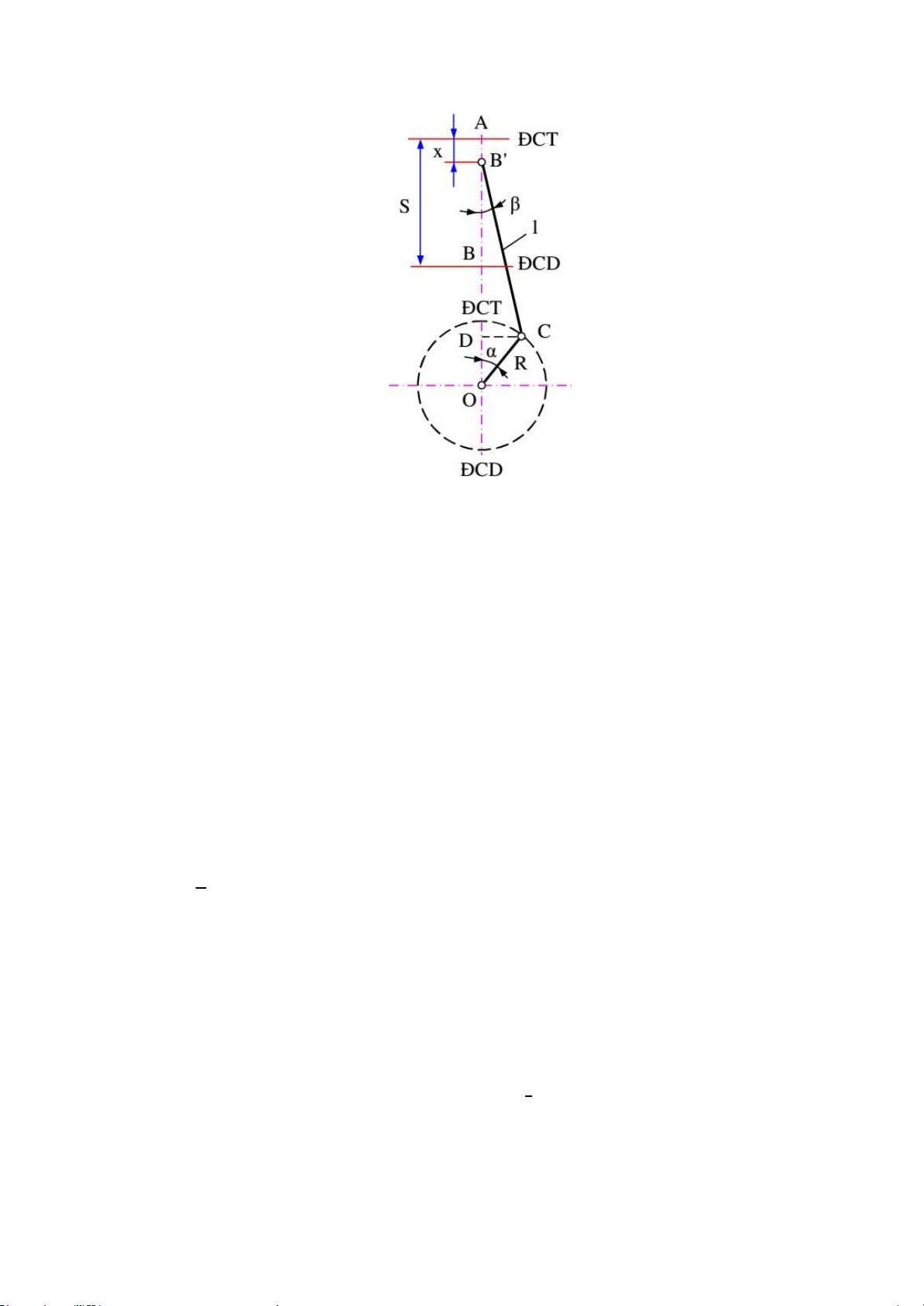
Động Dynamic diagram of piston - crankshaft - connecting rod mechanism
of the concentric structure
x – Displacement of piston calculated from TDC according to crankshaft rotation angle L – Connecting rod length
R – Rotation radius of the crankshaft α – Rotation angle of the crankshaft β
– Angle of deviation between the centerline of the connecting rod and
the centerline of the cylinder R
Let λ = be the structural parameter (λ = 0.24 ÷ 0.34). L
Applying the approximate formula to the concentric structure, we have:
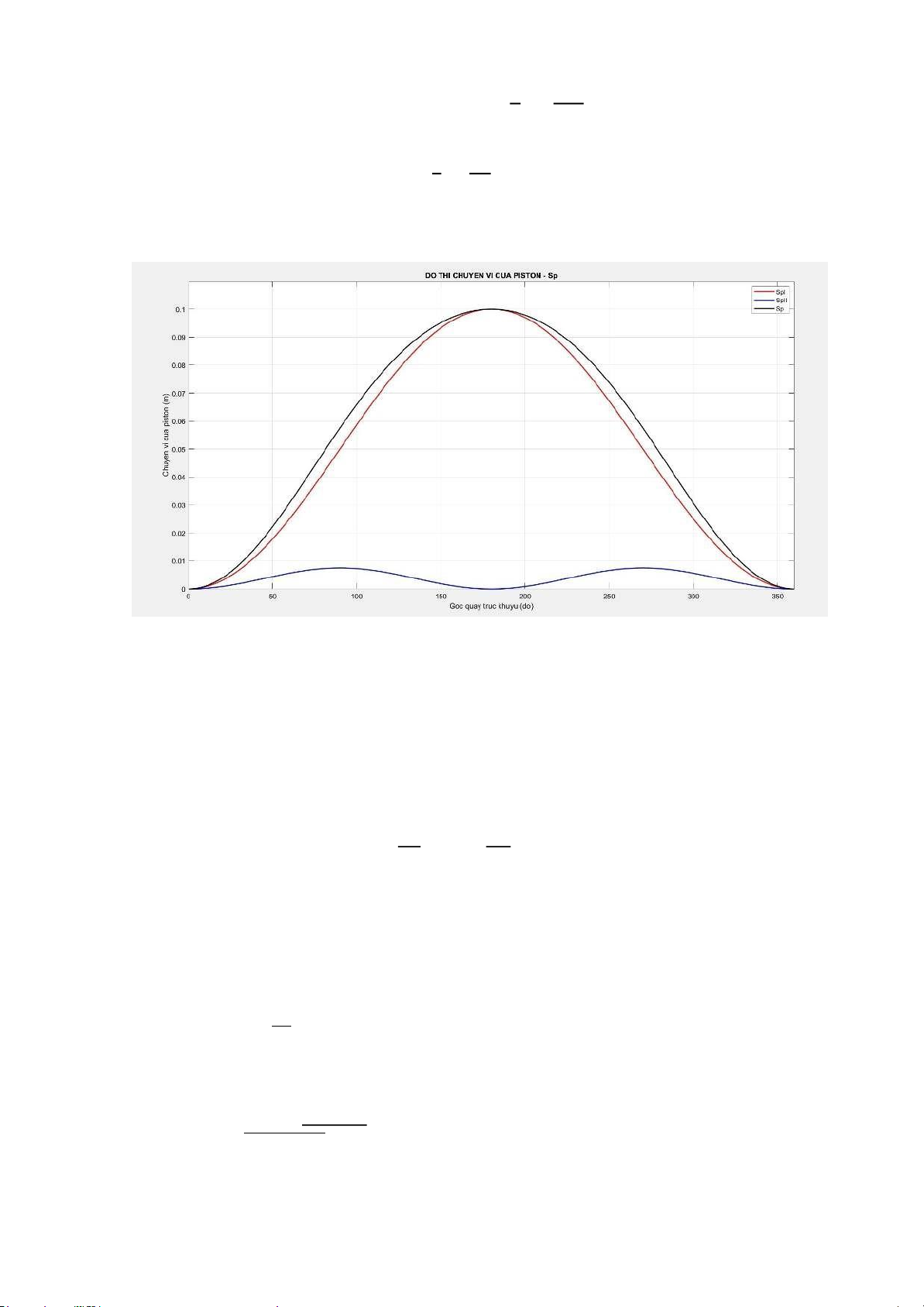
When the crankshaft rotates an angle, the piston moves a distance Sp compared to its initial position (ĐCT). λ Sp = R. [(1 − cos α) + (1 − cos 2α)] 4 With:
𝝋: Structural parameters of the engine. Choose λ = 0,30 𝝋 S/2
L: Is the length of the connecting rod. 𝝋 = = lOMoARcPSD| 36991220 = 0.17(𝝋) 𝝋 0,25 S 0.1
R: Crankshaft turning radius. R = = = 0.05(m) 2 2
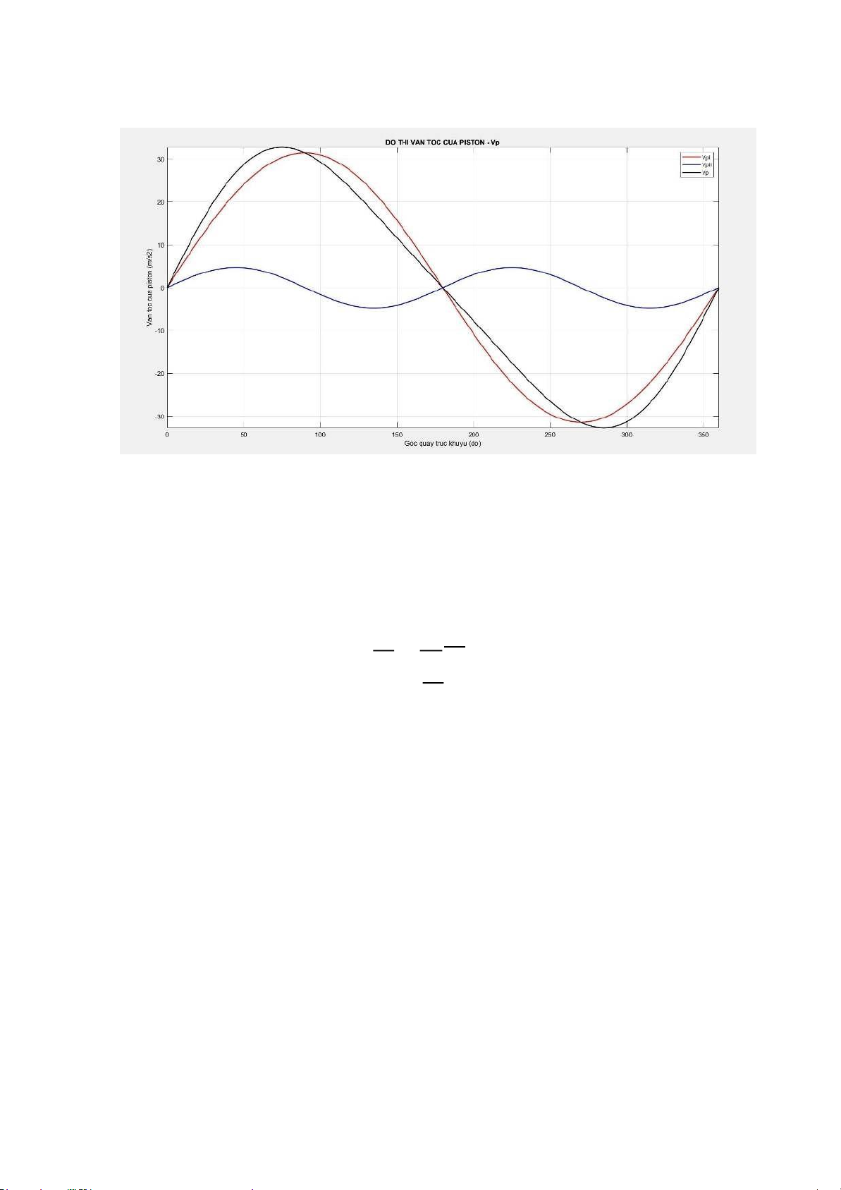
Using MATLAB, we can draw the piston displacement graph as follows: 2. Piston speed
Differentiating the displacement expression over time will yield the piston motion speed equation: dx dα dt = Vp; dt = ω λ
Vp = R. ω. (sin(α) + sin(2α)) 2 Average piston speed: V tb
Sn = 2 . R. ω, (m/s): Average piston speed = 30 π 2.π.n 2.π.6000 ω = =
= 200 𝝋, (rad/s): Angular velocity of the 60 60 crankshaft
Using MATLAB, we can draw the piston displacement graph as lOMoARcPSD| 36991220 follows: 3. Piston acceleration
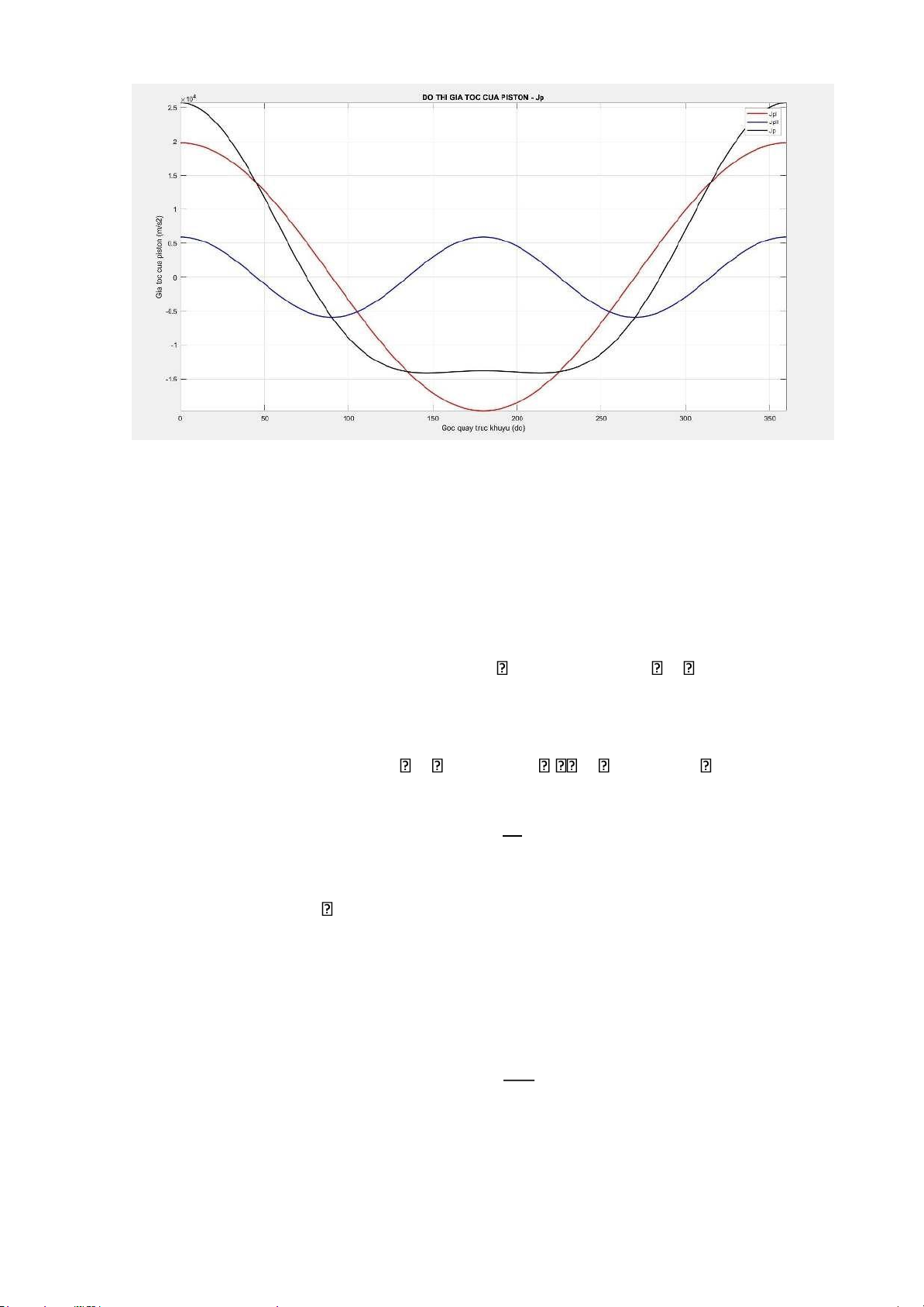
Differentiating the velocity expression with respect to time, we have the piston acceleration formula: jp = dv = dv . dα = dv dt dα dt da . ω
jp = R. ω2(cos(α) + λ cos(2α))
Using MATLAB, we can draw the piston displacement graph as follows: lOMoARcPSD| 36991220
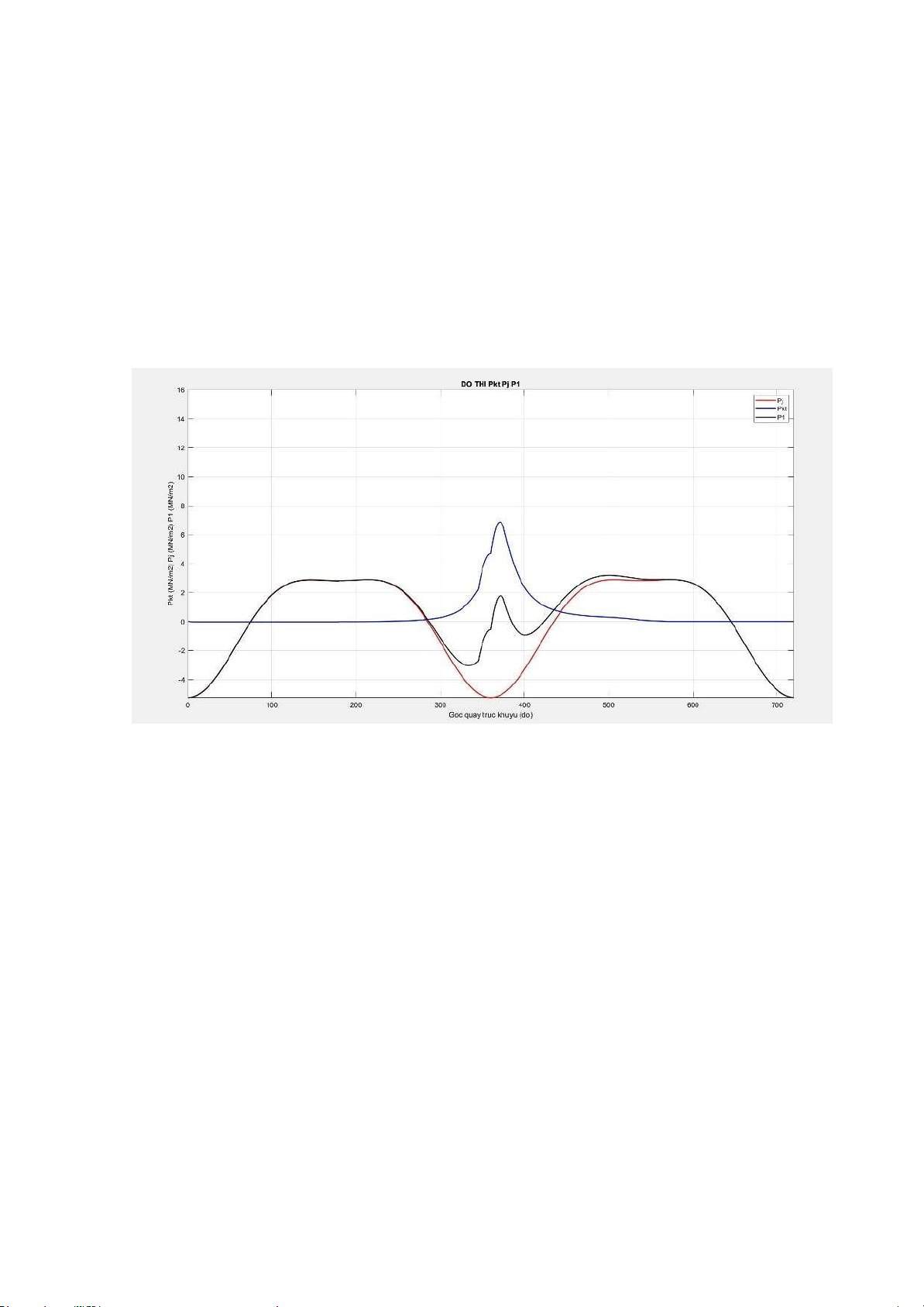
II. Dynamics of the crankshaft - connecting rod mechanism 1. Pneumatic force
From the indicated work graph, draw the pneumatic force graph Pkt dựa based
on the pressure values available in the P – indicated work graph and redraw
according to the crankshaft rotation angle Intake process: = 3°, 180°] pkt = pa
Compression process: = 180°, 360° = 180°, 345° pkt = pa. (Va) n1 Vc𝝋
Expansion process: goes from the end point of the combustion process on the indicator diagram.
𝝋 = [360°, 540° − 𝝋1] = [360°, 488°] Vz𝝋𝝋 n2 pkt = pz𝝋𝝋. ( ) Vb𝝋
Exhaust procces: α = [540°, 720°] pkt = pr lOMoARcPSD| 36991220
The correction segments of the pkt pneumatic force graph are similar to those on
the P - V indicator work graph, but instead of adjusting according to V, the
pneumatic force graph will be corrected according to .
2. Inertial force of moving parts
Mass of the crankshaft - connecting rod mechanism
Mass of piston group (mass of selected moving parts: mnp = 20 (g/cm2) (aluminum alloy piston)
Mass of the crankshaft (rotating parts) Choose: mk = 20 (g/cm2)
Mass of the connecting rod group
We can choose: mtt = 20 (g/cm2)
To simplify the calculation and its error is not significant, we choose the method
of using mass instead. The replacement volume is calculated according to the formula: L − a a ma = mtt. ( ) ; mb = mtt. L L
According to the empirical formula: 1 2 ma = . mtt ; mb = . mtt 3 3
Translational mass of the crankshaft - connecting rod mechanism: mt = mnp + mA
Rotational mass of the connecting rod crankshaft mechanism: mr = mk + mB
Inertial force (straightening) of a reciprocating mass
pj = −mt. R. ω2. (cos(α) + λ. cos(2α)) (MN/m2), with follow each process similar to
the pneumatic force 𝝋𝝋𝝋 . lOMoARcPSD| 36991220
Inertial force (centrifugal force) of rotating mass pk pk
= −mr. R. ω2(MN/m2) Total force p1 is the combined force of atmospheric force and inertial force
calculated according to the
formula: p1 = pkt + pj
Using MATLAB, we can draw the graph of forces 𝝋𝝋𝝋, 𝝋𝝋, 𝝋𝝋 as follows: Draw a P-V graph % THONG SO CO BAN D = 0.89; %(dm) S = 1; %(dm) R = S/2; %(dm) T = 13; Vd = 0.681; %(lit)
Sp = pi*D^2/4; %Dien tich piston lamda = 0.32; P0 = 0.1013 %MN/m Pa = 0.8*P0; %MN/m Pr = 0.11; Pz = 8.95; Pc = 2.72; Pb = 0.38; ro = 1;
Vc = Vd/(T-1);% c: cuoi qtrinh nen
Vz = ro*Vc;% z: cuoi qtrinh chay lOMoARcPSD| 36991220 %Va = Vd+Vc w = (pi*200) %rad Fp = (pi*(D^2))/4;
Va = 0.74 ; %Don vi the tich: lit % a: cuoi qtrinh nap Vb = Va;
% b: cuoi qtrinh gian no Vr = Vc; % r: cuoi qtrinh thai
n1 = 1.37; %2.3.2.4.Chi so nen da bien trung binh n2 =
1.23; %2.3.4.3.Chi so dan no da bien trung binh n = 6000; %vong/phut mpg = 13.35; %don vi g/cm2 mcr = 17.8; mcrsh = 17.8; mA = 0.4 * mcr; mB = 0.6 * mcr; mj = mA + mpg; mr = mB + mcrsh; % TINH TOAN CO BAN grid on
Xa = R*(1-cosd(180) + (lamda/4).*(1-cosd(2.*180))); Va = Xa*Sp + Vc; % (lit) % HIEU CHI THAI - NAP ahc1 = [0 5 10]; phc1 = [Pr 0.07 Pa]; a1 = linspace(0,10,1000);
X1 = R*(1-cosd(a1) + (lamda/4).*(1-cosd(2.*a1))); V1 = X1*Sp + Vc;
P1 = interp1(ahc1,phc1,a1, 'spline'); % QUA TRINH NAP a2 = linspace(10,180,1000); X2 = R*(1-cosd(a2)+(lamda/4)*(1- cosd(2*a2))); V2 = X2*Sp+Vc;
P2 = linspace(Pa,Pa,1000);%MN/m2 % QUA TRINH NEN a3 = linspace(180,350,1000);
X3 = R*(1-cosd(a3)+(lamda/4)*(1-cosd(2*a3))); V3 = X3*Sp+Vc; P3 = Pa*((Va./V3).^n1);%MN/m2 % HIEU CHINH NEN - CHAY Pz1 = 0.85*Pz; Pcc =(Pz1-Pc)/3 + Pc; ahc4 = [350 353 360]; phc4 = [max(P3) 3.15 Pcc]; a4 = linspace(350,360,1000);
X4 = R*(1-cosd(a4)+(lamda/4)*(1-cosd(2*a4))); V4=X4*Sp+Vc;
P4 = interp1(ahc4,phc4,a4, 'spline'); % Diem z” lOMoARcPSD| 36991220
X41 = R*(1-cosd(375) + (lamda/4).*(1-cosd(2.*375))); V41 = X41*Sp + Vc; % QUA TRINH GIAN NO a6 = linspace(375,500,1000);
X6 = R*(1-cosd(a6) + (lamda/4).*(1-cosd(2.*a6))); V6 = X6.*Sp + Vc; P6 = Pz.*(Vz./V6).^n2; % HIEU CHINH CHAY - GIAN NO ahc5=[360 365 375]; phc5=[Pcc 7 max(P6)]; a5=linspace(360,375,1000);
X5 = R*(1-cosd(a5) + (lamda/4).*(1-cosd(2.*a5))); V5 = X5.*Sp + Vc;
P5 = interp1(ahc5,phc5,a5,'spline'); % HIEU CHINH GIAN NO - THAI % Diem b’ Pb = min(P6); % Diem b” Vbb = Va; Pbb =(Pb-Pr)/2+Pr; ahc7 = [500 540 580]; phc7 = [Pb Pbb Pr]; a7 = linspace(500,580,100);
X7 = R*(1-cosd(a7) + (lamda/4).*(1-cosd(2.*a7))); V7 = X7.*Sp + Vc;
P7 = interp1(ahc7,phc7,a7,'spline'); % QUA TRINH THAI a8 = linspace(580,720,1000);
X8 = R*(1-cosd(a8) + (lamda/4).*(1-cosd(2.*a8))); V8 = X8*Sp + Vc; P8 = linspace(Pr,Pr,1000);
V = [V1 V2 V3 V4 V5 V6 V7 V8];
P = [P1 P2 P3 P4 P5 P6 P7 P8]; figure(1) % DO THI P-V
plot(V1,P1,'g','linewidth',1.5,'Color','black'); hold on
plot(V2,P2,'b','linewidth',1.5,'Color','black'); hold on
plot(V3,P3,'y','linewidth',1.5,'Color','black'); hold on
plot(V4,P4,'r','linewidth',1.5,'Color','black'); hold on
plot(V5,P5,'m','linewidth',1.5,'Color','black'); hold on
plot(V6,P6,'k','linewidth',1.5,'Color','black'); hold on lOMoARcPSD| 36991220
plot(V7,P7,'c','linewidth',1.5,'Color','black'); hold on
plot(V8,P8,'linewidth',1.5,'Color','black');
hold on title('DO THI P-V'); xlabel('The
tich V (dm3)'); ylabel('Ap suat P (MN/m2)'); grid on hold on clearvars; %% Cac thong so ban dau S = 1; % S/D=1.12, don vi dm D = 0.89; R = S/2; %dm lambda = 0.30; Fp = (pi*(D^2))/4;
Va = 0.74 ; %Don vi the tich: lit % a: cuoi qtrinh nap
Vc = 0.05; % c: cuoi qtrinh nen
Vz = 0.05; % z: cuoi qtrinh chay Vb = Va;
% b: cuoi qtrinh gian no Vr = Vc; % r: cuoi qtrinh thai n1 = 1.37;
%2.3.2.4.Chi so nen da bien trung binh
n2 = 1.23; %2.3.4.3.Chi so dan no da bien trung binh P0 = 0.1013; %2.2.1.Don vi ap suat: MN/m^2 Pa = 0.08104; %2.2.5 Pc = 2.72; %2.3.3.10 Pz = 8.95; %2.3.3.10 Pb = 0.38; %2.3.4.5 Pr = 0.11; %2.2.6 n = 6000; %vong/phut w = (pi*n)/30; %rad/s mpg = 13.35; %don vi g/cm2 mcr = 17.8; mcrsh = 17.8; mA = 0.4 * mcr; mB = 0.6 * mcr; mj = mA + mpg; mr = mB + mcrsh; %% ve do thi cong chi thi % hieu chinh rr'
a1hc = linspace (0,5,100); % dong muon xupap thai = 3 x1hc
= R.*((1-cosd(a1hc))+(lambda/4).*(1-cosd(2.*a1hc))); V1hc = x1hc*Fp + Vc; Vr1 = max (V1hc);
Prr1 = linspace (Pr,Pa,100); % khoang ap suat trong doan hieu chinh
Vrr1 = linspace (Vc,Vr1,100); % khoang the tich trong doan hieu chinh
P1hc = interp1 (Vrr1,Prr1,V1hc,'spline'); lOMoARcPSD| 36991220 % qua trinh nap a1 = linspace (5,180,100);
x1 = R.*((1-cosd(a1))+(lambda/4).*(1-cosd(2.*a1))); Fp = (pi*(D^2))/4; V1 = x1*Fp + Vc; P1 = linspace (Pa,Pa,100);
% qua trinh nen (goc danh lua som = 15) % doan 1 a2 = linspace (180,345,100);
x2 = R.*((1-cosd(a2))+(lambda/4).*(1-cosd(2.*a2))); V2 = x2*Fp + Vc; P2 = Pa.*(Va./V2).^n1; % qua trinh chay - gian no
% hieu chinh doan c'-c" a2hc = linspace (345,360,100);
x2hc = R.*((1-cosd(a2hc))+(lambda/4).*(1-cosd(2.*a2hc))); V2hc = x2hc*Fp + Vc; Pchc = Pa.*(Va./V2hc).^n1; % xac dinh toa do diem c' Vc1 = max (V2hc); Pc1 = min (Pchc); % xac dinh toa do diem c" Pz1 = Pz; % z1 la diem z' Pcz1 = Pz1 - Pc; Pc2 = Pcz1/3 + Pc; Vc2 = Vc; % ve doan c'-c"
Vc1c2 = linspace (Vc1,Vc2,100);
Pc1c2 = linspace (Pc1,Pc2,100);
P2hc = interp1(Vc1c2,Pc1c2,V2hc,'spline'); % hieu chinh c"-z" a3hc = linspace(360,375,100); x3hc = R.*((1- cosd(a3hc))+(lambda/4).*(1- cosd(2.*a3hc))); VZ = x3hc*Fp + Vc; PZ= Pz.*(Vz./VZ).^n2; % xac dinh diem z" Vz2 = max (VZ); Pz2 = min (PZ); % xac dih diem zhc azhc = 374;
xzhc = R.*((1-cosd(azhc))+(lambda/4).*(1-cosd(2.*azhc))); Vzhc = xzhc*Fp + Vc; Pzhc = Pz.*( Vz./Vzhc).^n2; % ve doan c"-z" Vz1z2 = [Vc2,Vzhc,Vz2]; lOMoARcPSD| 36991220 Pz1z2 = [Pc2,Pzhc,Pz2]; V3hc = linspace(Vc2,Vz2,100);
P3hc = interp1(Vz1z2,Pz1z2,V3hc,'spline'); % gian no a3 = linspace (375,488,100);
x3 = R.*((1-cosd(a3)+(lambda/4).*(1-cosd(2.*a3)))); V3 = x3*Fp + Vc; P3 = Pz.*(Vz./V3).^n2; % qua trinh thai % hieu chinh b'b"
a4hc = linspace (488,540,100); %mo som xupap thai = 10
x4hc = R.*((1-cosd(a4hc))+(lambda/4).*(1-cosd(2.*a4hc))); V1b = x4hc*Fp + Vc; P1b = Pz.*(Vz./V1b).^n2; % xac dinh diem b' Vb1 = min (V1b); Pb1 = max (P1b); % xac dinh diem b" Pb2 = ((Pb-Pr)/3)+Pr; Vb2 = Va; % xac dinh bhc1 abhc1 = 500;
xbhc1 = R.*((1-cosd(abhc1))+(lambda/4).*(1- cosd(2.*abhc1))); Vbhc1 = xbhc1*Fp + Vc; Pbhc1 = Pz.*(Vz./Vbhc1).^n2; % ve doan b'b" Vb1b2 = [Vb1,Vbhc1,Vb2]; Pb1b2 = [Pb1,Pbhc1,Pb2]; V4hc = linspace(Vb1,Va,100);
P4hc = interp1(Vb1b2,Pb1b2,V4hc,'spline'); % hieu chinh b" a5hc = linspace(540,570,100);
x5hc = R.*((1-cosd(a5hc))+(lambda/4).*(1-cosd(2.*a5hc))); V2b = x5hc*Fp + Vc; %xac dinh diem b''' Pb3 = Pr; Vb3 = min(V2b); %xac dinh diem bhc2 abhc2 = 1; xbhc2 = R.*((1-
cosd(abhc2))+(lambda/4).*(1cosd(2.*abhc2))); Vbhc2 = xbhc2*Fp + Vc; Pbhc2 = 0.225; % ve doan cong sau b" Vb2b4 = [Vb2,Vbhc2,Vb3]; lOMoARcPSD| 36991220 Pb2b4 = [Pb2,Pbhc2,Pb3]; V5hc = linspace(Vb2,Vb3,100);
P5hc = interp1(Vb2b4,Pb2b4,V5hc,'spline'); % doan cuoi a4 = linspace (570,720,100);
x4 = R.*((1-cosd(a4))+(lambda/4).*(1-cosd(2.*a4))); V4 = x4*Fp + Vc; P4 = linspace (Pr,Pr,100);
%%%%%%%%%%%%%%%%%%%%%%%%%%%%%%% % do thi cong P-V
atong = [a1hc,a1,a2,a2hc,a3hc,a3,a4hc,a5hc,a4]; jtong
= R*(w^2).*(cosd(atong)+lambda.*cosd(2.*atong));
Vtong = [V1hc,V1,V2,V2hc,VZ,V3,V1b,V2b,V4];
Ptong = [P1hc,P1,P2,P2hc,P3hc,P3,P4hc,P5hc,P4]; %% do thi P-phi Pj P1 figure(2); Pj = (-mj.*jtong)*(10^-6);% Pkt = (Ptong-0.1);
plot (atong,Pj,'r','linewidth',1.5); hold on
plot (atong,Pkt,'b','linewidth',1.5); P1 = Pkt + Pj; plot
(atong,P1,'k','linewidth',1.5); axis([0 720 -6 10]); grid on;
title('DO THI Pkt Pj P1'); xlabel('Goc quay
truc khuyu (do)'); ylabel('Pkt (MN/m2) Pj (MN/m2) P1 (MN/m2)'); legend('Pj','Pkt','P1'); %% do thi dong hoc adh = [a1hc,a1,a2,a2hc]; %chuyen vi cua piston SpI = 0.1*R.*(1-cosd(adh));
SpII = 0.1*R.*((lambda/4).*(1-cosd(2.*adh))); Sp = SpI + SpII; figure(3);
plot (adh,SpI,'r','linewidth',1.5); hold on;
plot (adh,SpII,'b','linewidth',1.5); hold on;
plot (adh,Sp,'k','linewidth',1.5); axis([0 360 0 0.11]);
title('DO THI CHUYEN VI CUA PISTON - Sp');
xlabel('Goc quay truc khuyu (do)');
ylabel('Chuyen vi cua piston (m)'); legend('SpI','SpII','Sp'); grid on; lOMoARcPSD| 36991220 %van toc cua piston VpI = 0.1*R*w.*(sind(adh));
VpII = 0.1*R*w.*((lambda/2).*sind(2*adh)); Vp = VpI + VpII; figure(4);
plot (adh,VpI,'r','linewidth',1.5); hold on;
plot (adh,VpII,'b','linewidth',1.5); hold on;
plot (adh,Vp,'k','linewidth',1.5);
axis([0 360 -40 40]); title('DO THI VAN
TOC CUA PISTON - Vp'); xlabel('Goc quay
truc khuyu (do)'); ylabel('Van toc cua piston (m/s2)'); legend('VpI','VpII','Vp'); grid on; %gia toc cua piston jI =
0.1*R*(w^2).*(cosd(adh)); jII =
0.1*R*(w^2).*(lambda.*cosd(2.*adh)); Jp = jI + jII; figure(5);
plot (adh,jI,'r','linewidth',1.5); hold on;
plot (adh,jII,'b','linewidth',1.5); hold on;
plot (adh,Jp,'k','linewidth',1.5);
axis([0 360 -20000 28000]); title('DO
THI GIA TOC CUA PISTON - Jp');
xlabel('Goc quay truc khuyu (do)');
ylabel('Gia toc cua piston (m/s2)'); legend('JpI','JpII','Jp'); grid on; clc;