Bài tập 4 Phân loại tuyến tính | Môn Trí tuệ nhân tạo - Đại học Sư phạm Kỹ thuật Thành phố Hồ Chí Minh

lOMoAR cPSD| 58778885
BÀI 4: PHÂN LOẠI TUYẾN TÍNH
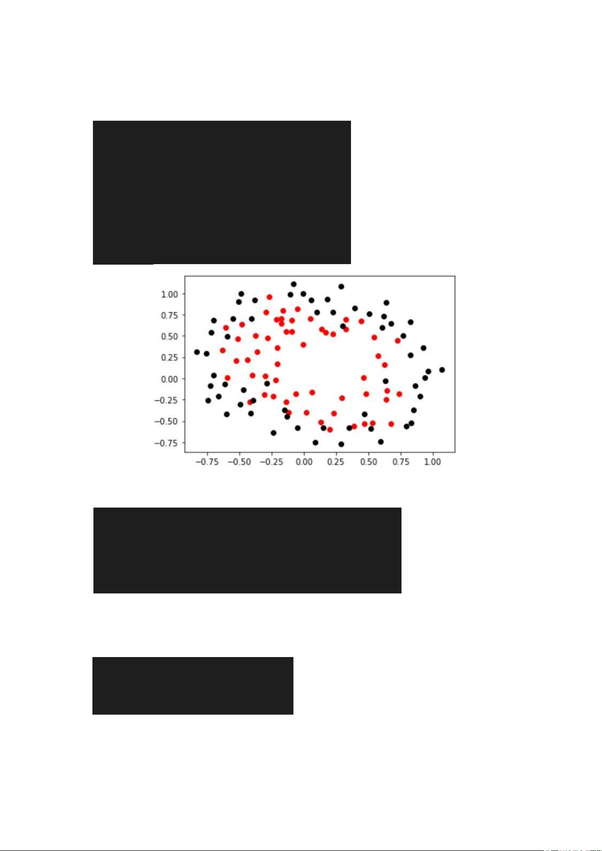
1. Biểu diễn dữ liệu
import pandas as pd import numpy as np
import matplotlib.pyplot as plt #doc du
lieu data = pd.read_csv("ex5data.txt", header=None, sep=",") x =
data.values[:,:-1] y = data.values[:,-1]
x_pos = x[y==1,:] x_neg = x[y==0,:] plt.scatter(x_pos[:,0], x_pos[:,1],c='r') plt.scatter(x_neg[:,0], x_neg[:,1],c='k')
2. Chuẩn hóa dữ liệu: scale dữ liệu, format kích thước dữ liệu
mean_x = x.mean(0,keepdims=1) std_x =
x.std(0,keepdims=1) x_ = (x-mean_x)/std_x x_ =
np.concatenate((np.ones((len(x_),1)),x_),1) y =
np.reshape(y,(len(y),1)) theta = np.random.rand(x_.shape[1],1)
3. Viết chương trình cho phép học các tham số của mô hình phân loại tuyến tính
# Hàm sigmoid def sigmoid(z):
return 1 / (1 + np.exp(-z)) def ham_h(x_, theta): lOMoAR cPSD| 58778885
return sigmoid(np.dot(x_,theta))
def cost_function_J(theta, x_, y): m = len(y)
h = ham_h(x_, theta) J = J = (-1 / m) * np.sum(y *
np.log(h) + (1 - y) * np.log(1 - h)) return J def
cap_nhat_theta(theta, x_, y, learning_rate): m = len(y) h = ham_h(x_, theta)
gradients = (1/m) * np.dot(x_.T, (h-y))
theta = learning_rate * gradients return theta
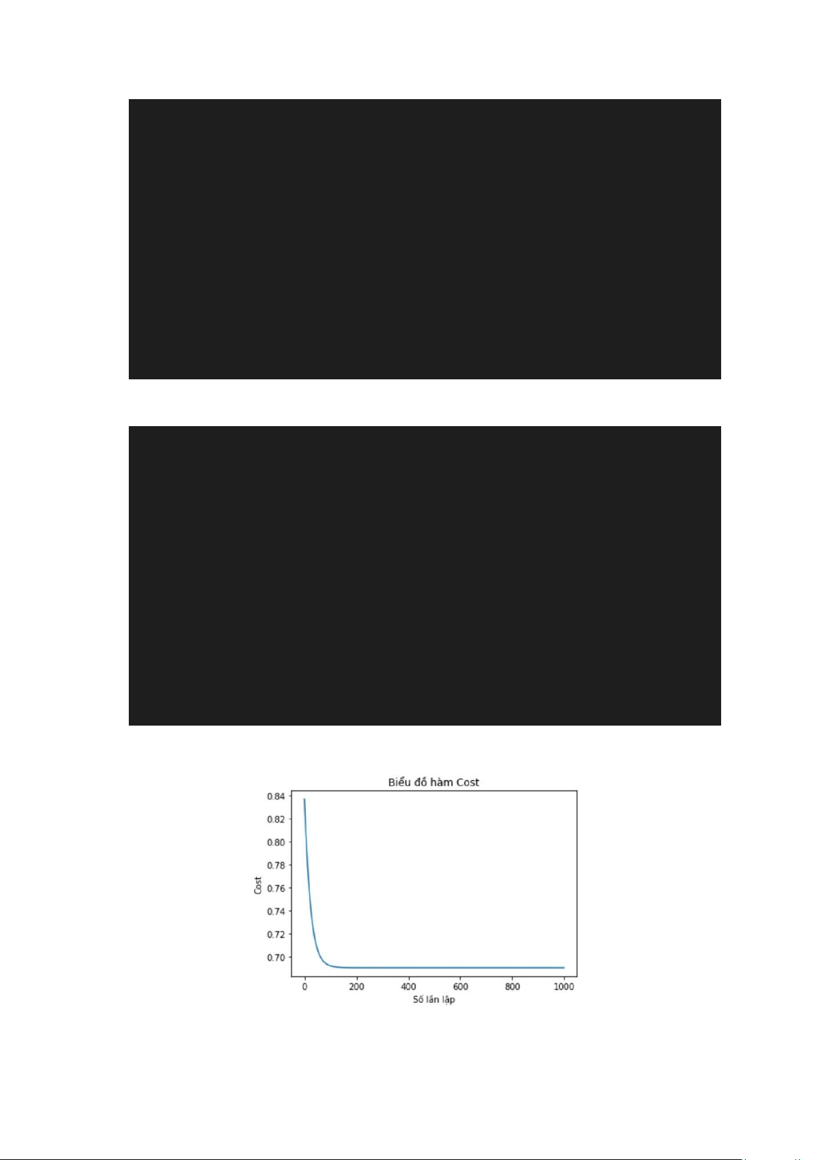
4. Tính J ở mỗi vòng lặp, và vẽ biểu đồ J ở các giá trị learning rate khác nhau
sau khi chạy hết các vòng lặp.
n = int(input('So vong lap: '))
learning_rate = float(input('Learning rate:
')) J_moi_vong_lap = [] for i in range(n):
theta = cap_nhat_theta(theta, x_, y, learning_rate)
J = cost_function_J(theta, x_, y)
J_moi_vong_lap.append(J) print(f'Lan lap {i+1}: Theta
= {theta.flatten()}, J = {J}') plt.plot(J_moi_vong_lap)
plt.xlabel('Số lần lặp') plt.ylabel('Cost') plt.title('Biểu đồ hàm Cost') plt.show()
* Vẽ biểu đồ J ở các giá trị learning rate khác nhau sau khi chạy hết các vòng
lặp (learning rate = 0.1 , số vòng lặp = 1000)
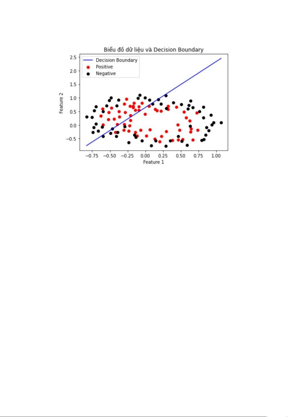
5. Biển diễn đường phân loại (decision boundary) học được và dữ liệu
trên cùng 1 hình ảnh. * Learning rate = 0.01, số vòng lặp = 1000 lOMoAR cPSD| 58778885