Bài tập Matlab Thông tin vô tuyến| Môn Thông tin vô tuyến| Trường Đại học Bách Khoa Hà Nội

Bài tập Matlab Thông tin vô tuyến
Sinh viên thực hiện : Hồ Anh Văn MSSV : 20102541
Giảng viên hướng dẫn : PGS.TS Nguyễn Văn Đức Exercise 1.1
% ====================================================================
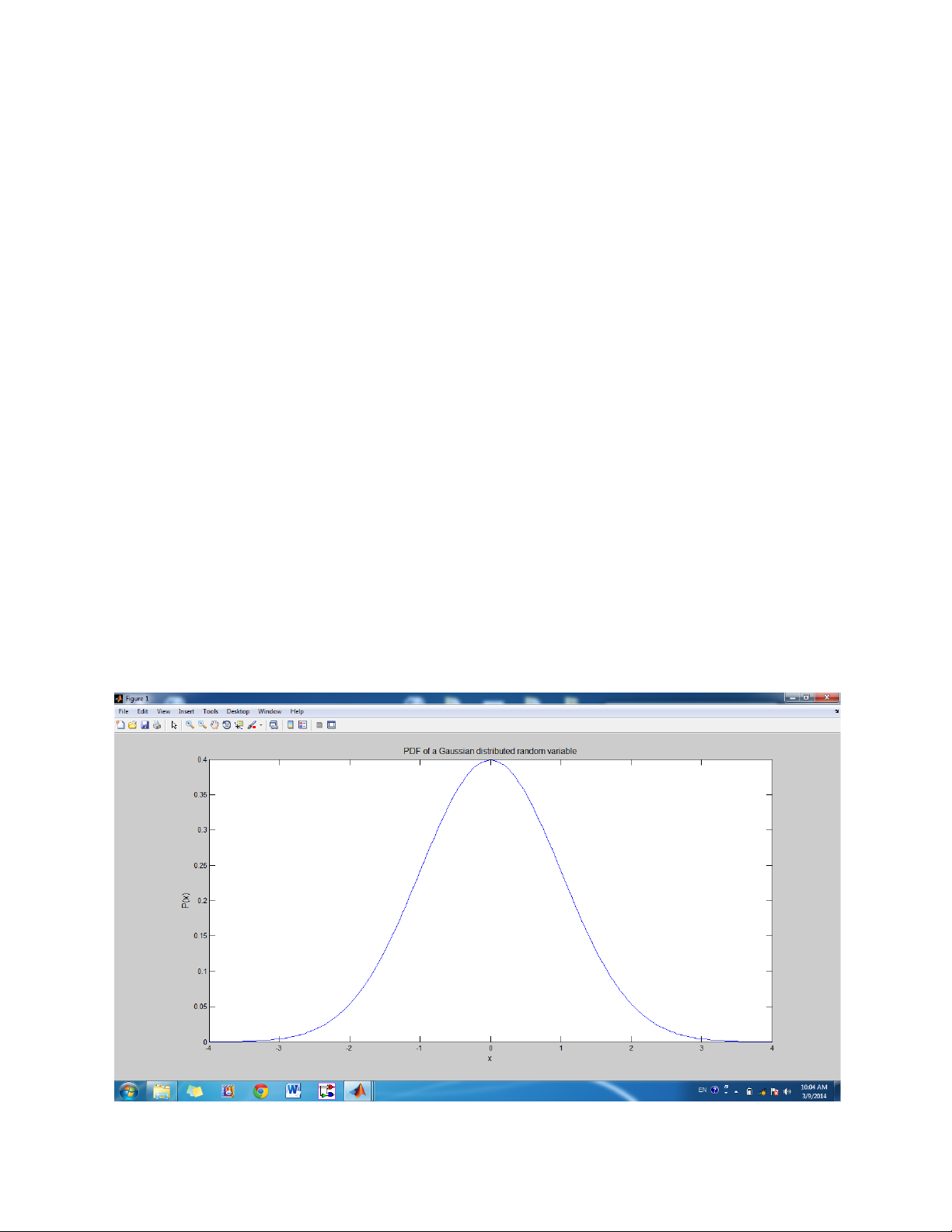
% Calculation of the probability density function (PDF) of a Gaussian % distributed random variable
% ====================================================================
t_a = 0.05; % Sampling interval x=-4:t_a:4; % Set x variable
% Calculation of the PDF of a Gaussian distributed random variable p=(1/sqrt(2*pi)*exp(-x.^2/2));
check=trapz(x,p); % Intergration of p
% Remark : the intergration of P(x) for -4<=x<=4 must be equal to 1 plot(x,p);
title('\fontsize{12}PDF of a Gaussian distributed random variable'); xlabel('x','Fontsize',12); ylabel('P(x)','FontSize',12) Exercise 1.2
% =============================================================
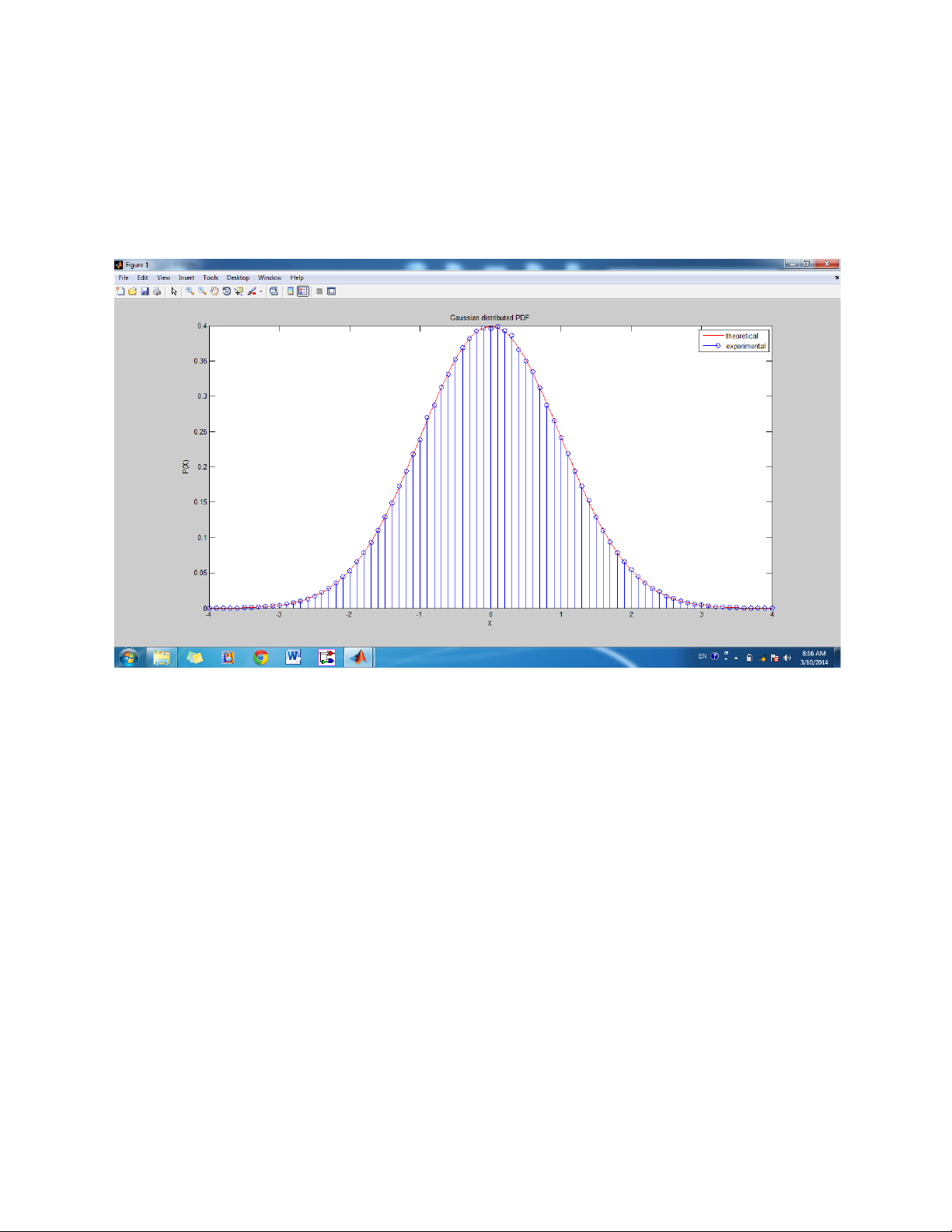
% Comparison of Gaussian distributed PDF with simulation result
% =============================================================
clear; % clear all available variables m_mu=0; % mean value sigma_mu=1; % variance
n=1000000; % length of the noise vector x=-4:0.05:4; % set x variable
p=(1/sqrt(2*pi)*sigma_mu)*exp(-(x-m_mu).^2/2*sigma_mu^2); % calculate the Gaussian distributed PDF
check=trapz(x,p) % the intergration of P(x) for -4<=x<=4 must equal 1 plot(x,p,'r'); hold on;
% =============================================================
% Generation o random vector,and calculate its distribution
% ============================================================= y=randn(1,n);
m=mean(y) % mean value of the process y
variance=std(y)^2 % variance of the process y x2=-4:0.1:4;
c=hist(y,x2); % calculated the history of the process y stem(x2,c/n/(x2(2)-x2(1)));
% the calcutation "c/n/(x2(2)-x2(1))"is to change from the history diagram % to the PDF
title('Gaussian distributed PDF'); xlabel('X'); ylabel('P(X)');
legend('theoretical','experimental'); hold off; Exercise 2.1
% =======================================
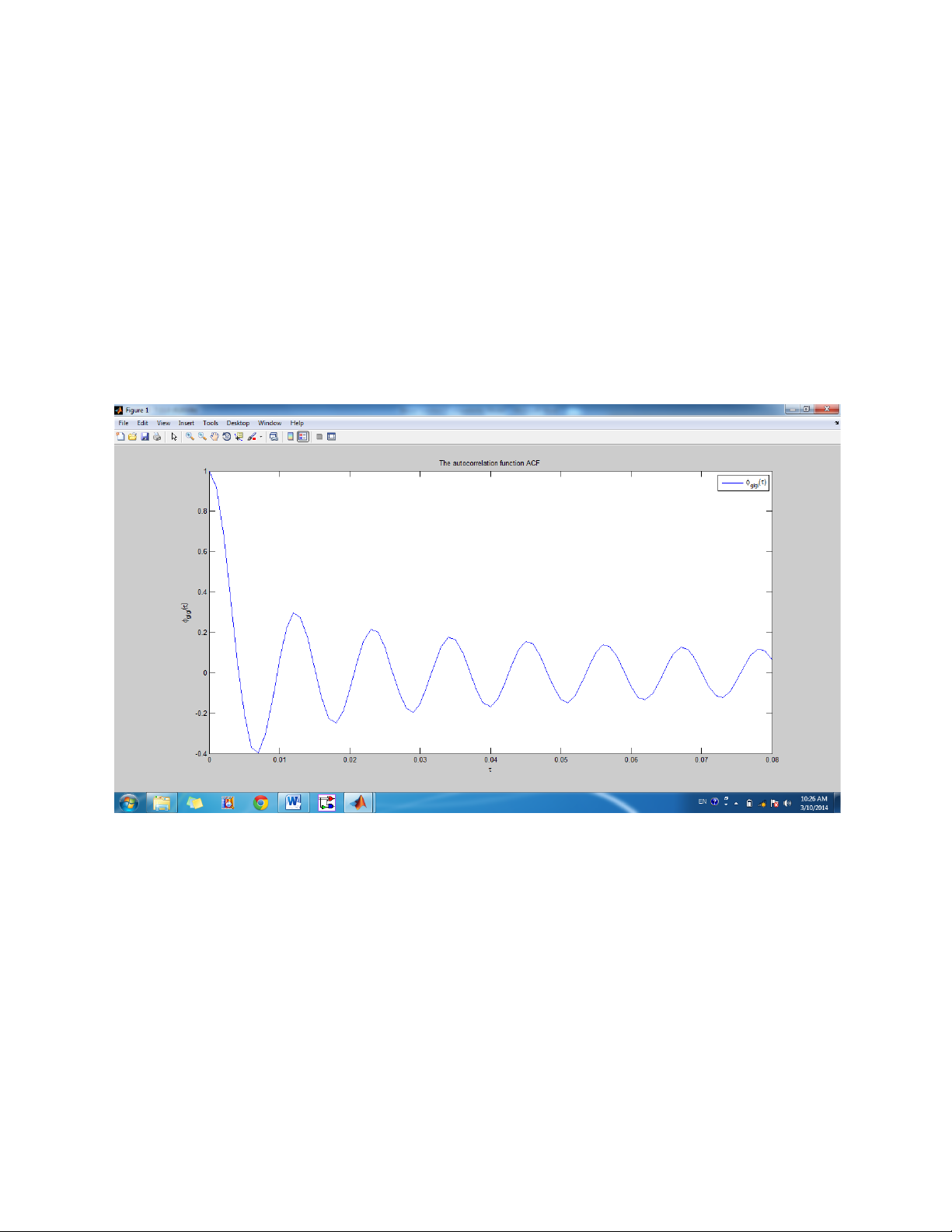
% Bessel function -> time autocorrelation function of the mobile channel
% ======================================= clear;
f_c=900e6; % the carrier frequency in Hz
c_0=3e8; % the speed of light in m/s
v=109.2e3/3600; % the mobile station’s speed in m/s
f_m=v*f_c/c_0; % the maximum Doppler frequency
ohm_p=2; % the total received power
t=0:0.001:0.08; % the time interval in second(s)
phi_gIgI=(ohm_p/2)*besselj(0,2*pi*f_m*t); % the autocorrelation function plot(t,phi_gIgI);
title('The autocorrelation function ACF'); xlabel('\tau'); ylabel('\phi_{gIgI}(\tau)'); legend('\phi_{gIgI}(\tau)');
phi_gIgI_0=(ohm_p/2)*besselj(0,0); Exercise 2.2 % ========================= % Doppler spectrum % ========================= clear;
f_c=900e6; % the carrier frequency in Hz
c_0=3e8; % the speed of light in m/s
v=109.2e3/3600; % the mobile station’s speed in m/s
f_m=v*f_c/c_0; % the maximum Doppler frequency
ohm_p=2; % the total received power
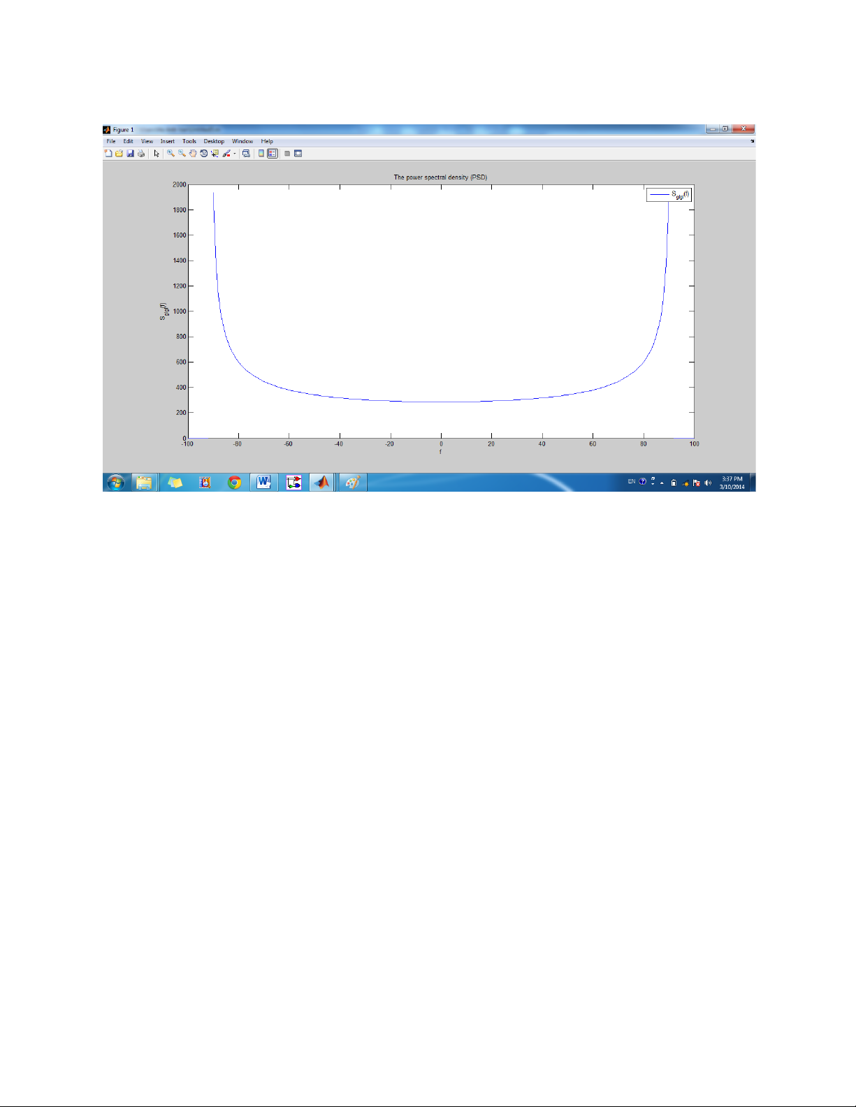
z=-100:1:100; % the time interval in second (s) for i=1:201; f=i-101; if abs(f)<=f_m
S_gIgI(i)=(ohm_p/2*pi*f_m)/sqrt(1-(f/f_m)^2); else S_gIgI(i)=0; end end plot(z,S_gIgI)
title('The power spectral density (PSD)') xlabel('f') ylabel('S_{gIgI}(f)') legend('S_{gIgI}(f)') Exercise 2.3
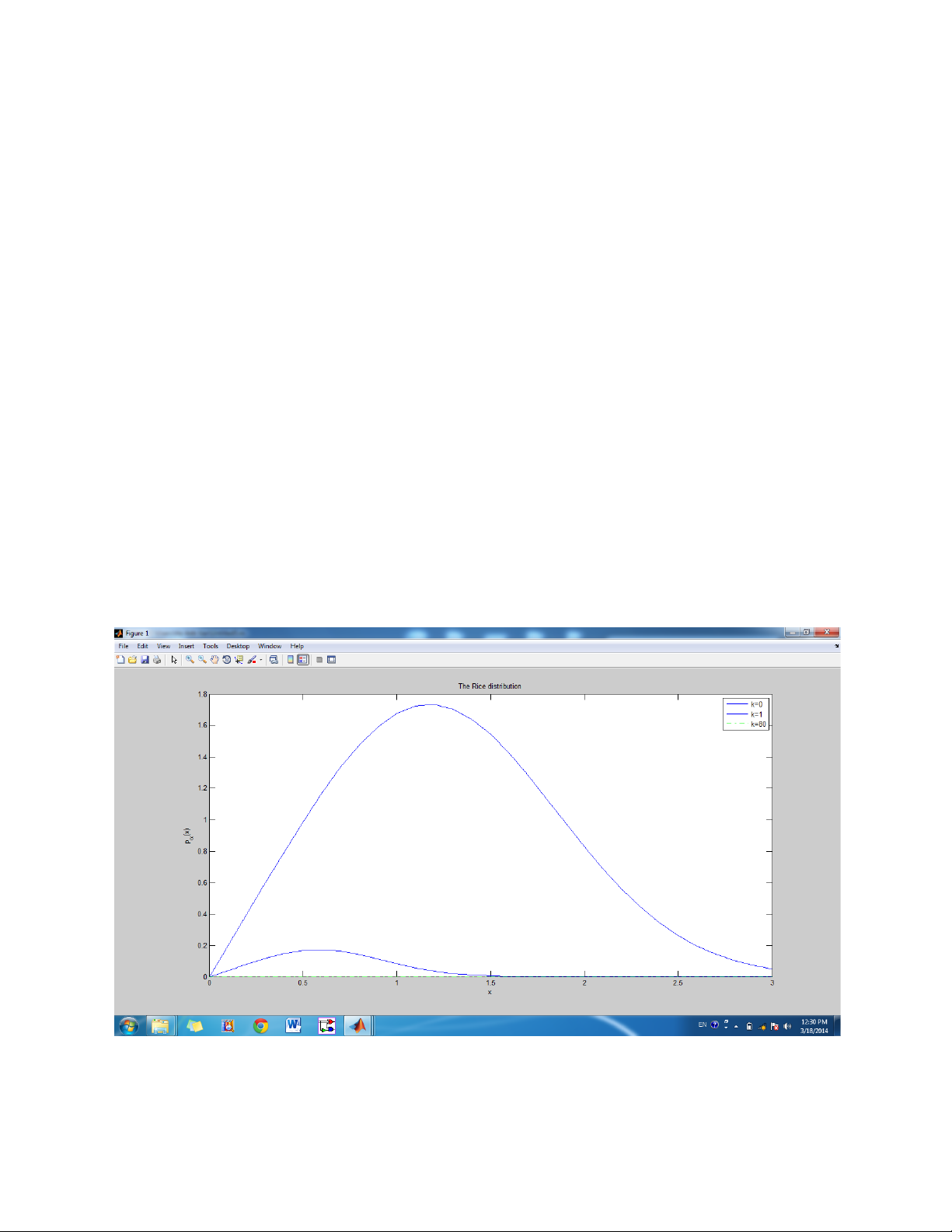
% =============================== % Distribution Rice
% =============================== clear; k0=0; k1=3; k2=80;
k=k0; % the rice of factor k=s^2/2b_0
x=0:0.1:3; % the time interval in seconds
ohm_p=1; % the total received power
p_elfa=(2.*x.*(k+1)/ohm_p).*exp(-k-((k+1).*x.^2/ohm_p)).*besseli(0,(2.*x.*sqrt( (k+1)/ohm_p))); plot(x,p_elfa) hold on k=k1;
p_elfa1=(2.*x.*(k+1)/ohm_p).*exp(-k-((k+1).*x.^2/ohm_p)).*besseli(0,(2.*x.*sqrt ((k+1)/ohm_p))); plot(x,p_elfa1) hold on k=k2;
p_elfa2=(2.*x.*(k+1)/ohm_p).*exp(-k-((k+1).*x.^2/ohm_p)).*besseli(0,(2.*x.*sqrt ((k+1)/ohm_p))); plot(x,p_elfa2,'g-.') title('The Rice distribution') xlabel('x') ylabel('p_{\alpha}(x)') legend('k=0','k=1','k=80') hold off Exercise 2.4
% ======================================
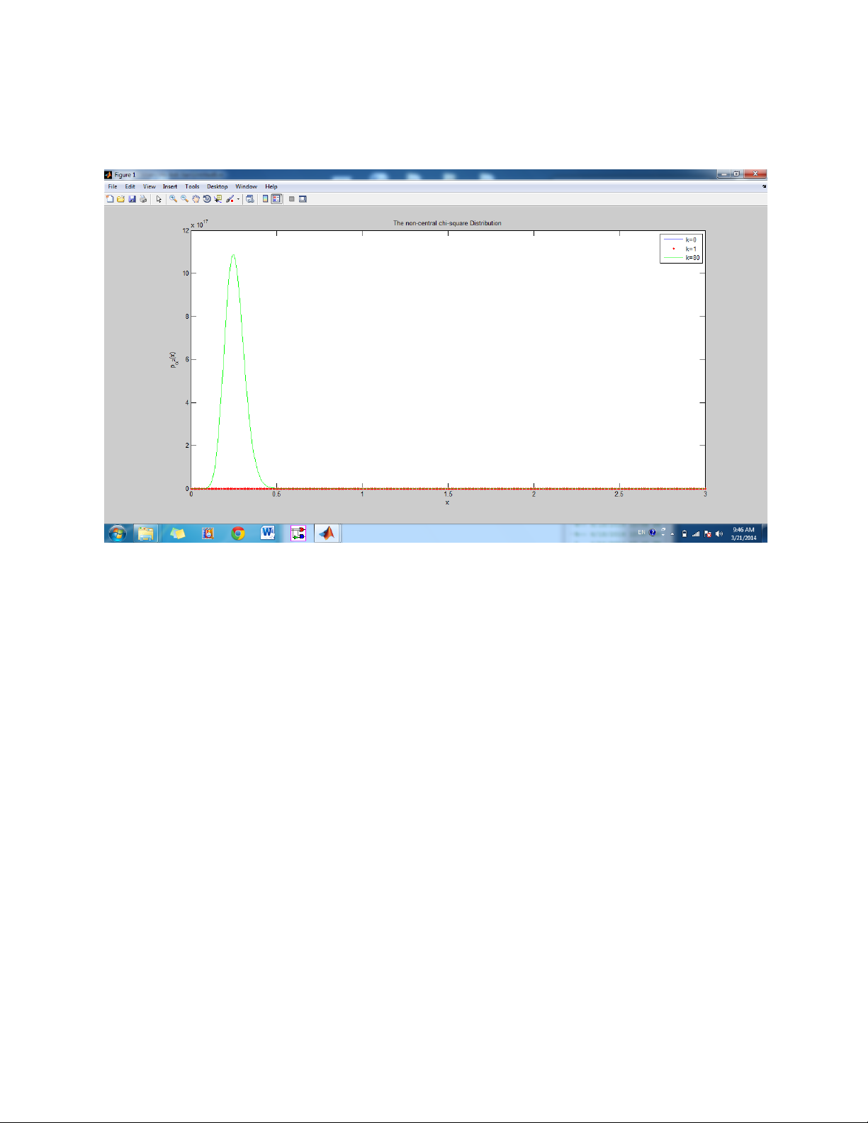
% The non-central chi/square Distribution
% ====================================== clear; k0=0; k1=3; k2=80;
k=k0; % the rice of factor k=s^2/2b_0
x=0:0.01:3; % the time interval in second (s)
ohm_p=1; % the total received power
p_alpha=(k+1)/ohm_p.*exp(((-k-(k+1)).*x./ohm_p)).*besseli(0,(2*sqrt(k*(k+1).*x. /ohm_p))); plot(x,p_alpha) hold on k=k1;
p_alpha1=(k+1)/ohm_p.*exp(((-k-(k+1)).*x./ohm_p)).*besseli(0,(2*sqrt(k*(k+1).*x ./ohm_p))); plot(x,p_alpha1,'r.') k=k2;
p_alpha2=(k+1)/ohm_p.*exp(((-k-(k+1)).*x./ohm_p)).*besseli(0,(2*sqrt(k*(k+1).*x ./ohm_p))); plot(x,p_alpha2,'g-')
title('The non-central chi-square Distribution') xlabel('x') ylabel('p_{\alpha^2}(x)') legend('k=0','k=1','k=80') hold off Exercise 3.1
% ============================================
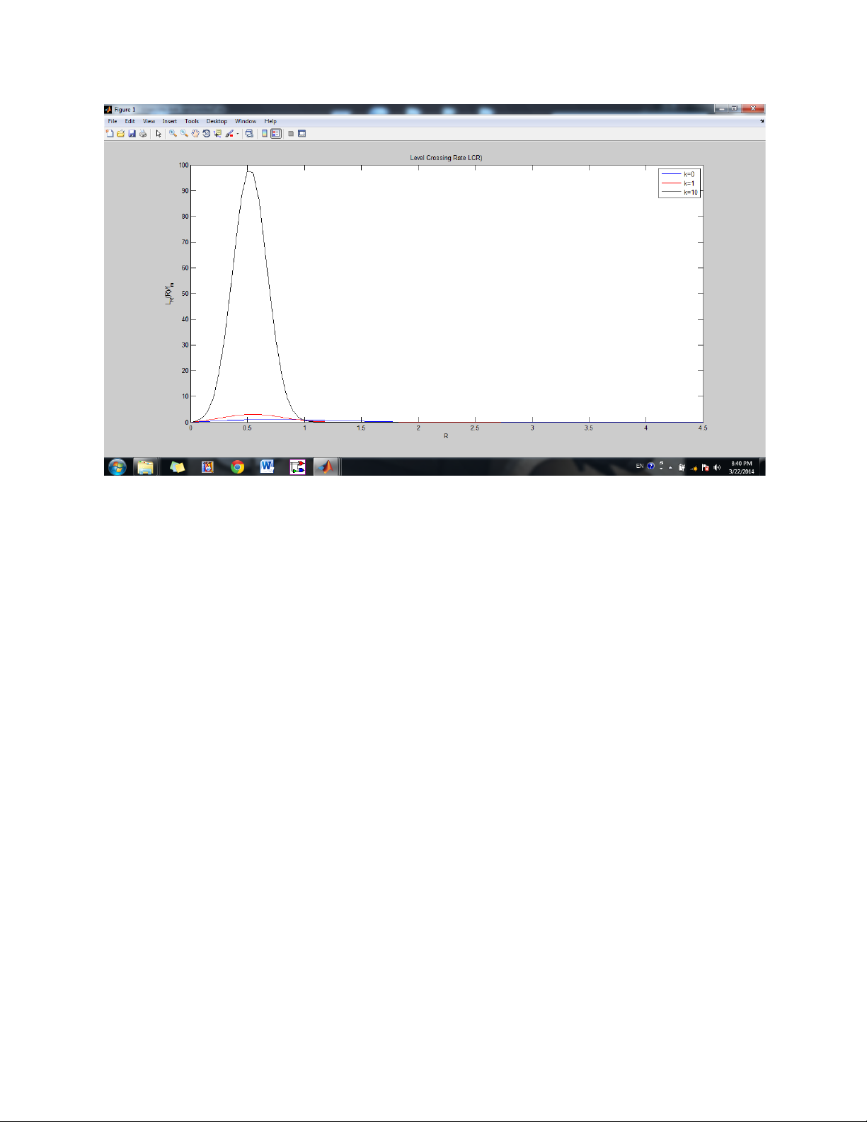
% The level crossing rate of the Rice processes
% ============================================ clear; k0=0; % the Rice factor k1=3; k2=10;
R=0:0.05:4.5; % the vector of amplitude levels
ohm_p=1; % the total received power rau=R./sqrt(ohm_p);
k=k0; % The Rice factor k=s^2/2b_0
L_R=sqrt(2*pi*(k+1)).*rau.*exp((-k-(k+1)).*rau.^2).*besseli(0,(2.*rau.*sqrt(k*( k+1)))); plot(R,L_R) hold on k=k1;
L_R1=sqrt(2*pi*(k+1)).*rau.*exp((-k-(k+1)).*rau.^2).*besseli(0,(2.*rau.*sqrt(k* (k+1)))); plot(R,L_R1,'r-') k=k2;
L_R2=sqrt(2*pi*(k+1)).*rau.*exp((-k-(k+1)).*rau.^2).*besseli(0,(2.*rau.*sqrt(k* (k+1)))); plot(R,L_R2,'k-')
title('Level Crossing Rate LCR)') xlabel('R') ylabel('L_R(R)/f_m') legend('k=0','k=1','k=10') hold off Exercise 3.2
% ==========================================
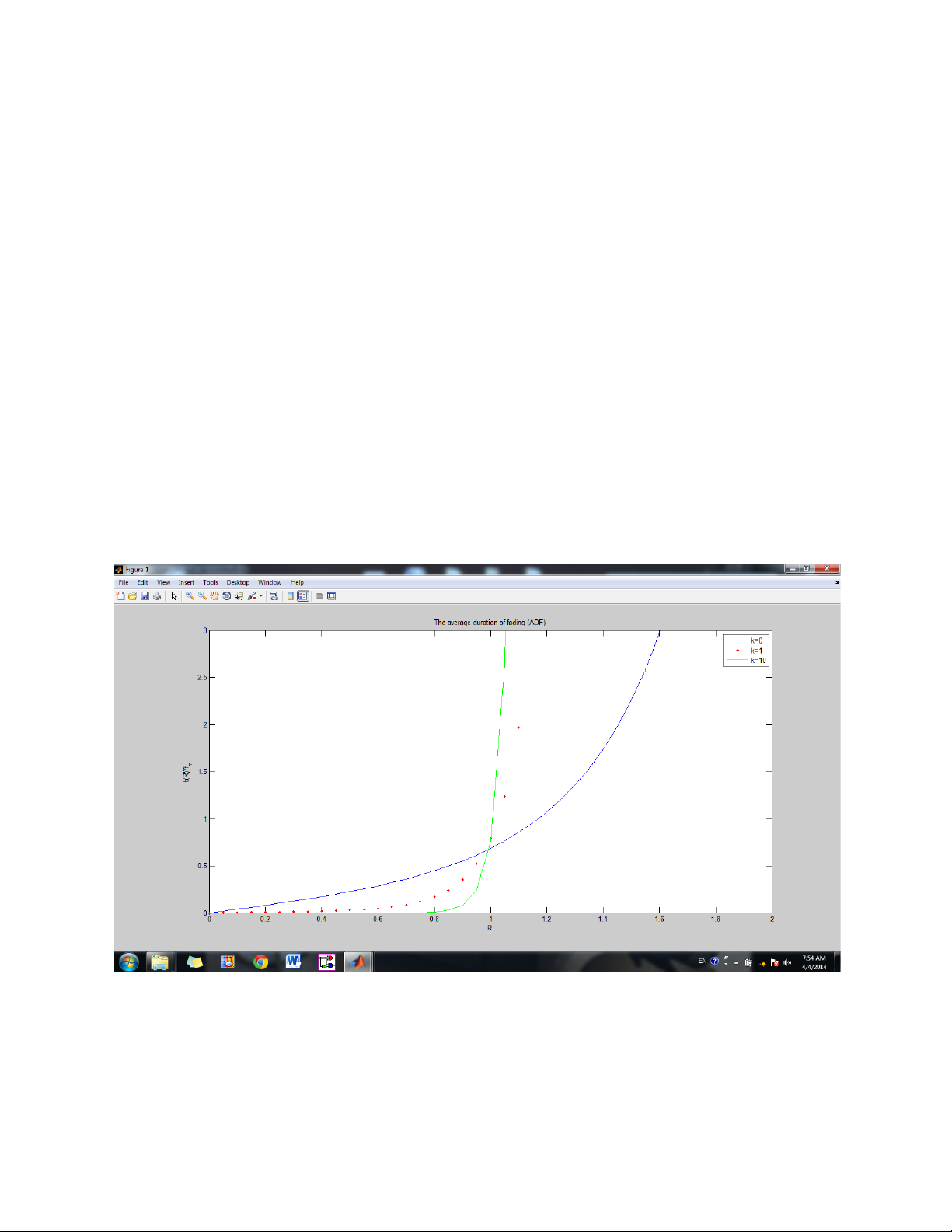
% The average duration of fading of the Rice processes
% ========================================== clear; k0=0; k1=3; k2=10; R=0.0001:0.05:4.51;
ohm_p=1; % the total received power rau=R./sqrt(ohm_p);
k=k0; % The Rice factor k=s^2/2b_0
L_R=sqrt(2*pi*(k+1)).*rau.*exp((-k-(k+1)).*rau.^2).*besseli(0,(2.*rau.*sqrt(k*( k+1)))); for r=0:0.05:4.5 x=linspace(0,r); a=0:0.05:r; i=length(a);
p=(2.*x.*(k+1)/ohm_p).*exp(-k-((k+1).*x.^2/ohm_p)).*besseli(0,(2.*x.*sqrt(k*(k+ 1)/ohm_p))); CDF(i)=trapz(x,p); end ADF=CDF./L_R; plot(R,ADF) hold on k=k1; % the rice factor k=s^2/2b_0
L_R1=sqrt(2*pi*(k+1)).*rau.*exp((-k-(k+1)).*rau.^2).*besseli(0,(2.*rau.*sqrt(k* (k+1)))); for r=0:0.05:4.5 x=linspace(0,r); a=0:0.05:r; i=length(a);
p=(2.*x.*(k+1)/ohm_p).*exp(-k-((k+1).*x.^2/ohm_p)).*besseli(0,(2.*x.*sqrt(k*(k+ 1)/ohm_p))); CDF1(i)=trapz(x,p); end ADF1=CDF1./L_R1; plot(R,ADF1,'r.') hold on k=k2;
L_R2=sqrt(2*pi*(k+1)).*rau.*exp((-k-(k+1)).*rau.^2).*besseli(0,(2.*rau.*sqrt(k* (k+1)))); for r=0:0.05:4.5 x=linspace(0,r); a=0:0.05:r; i=length(a);
p=(2.*x.*(k+1)/ohm_p).*exp(-k-((k+1).*x.^2/ohm_p)).*besseli(0,(2.*x.*sqrt(k*(k+ 1)/ohm_p))); CDF2(i)=trapz(x,p); end ADF2=CDF2./L_R2; plot(R,ADF2,'g-') axis([0 2 0 3])
title('The average duration of fading (ADF)') xlabel('R') ylabel('t(R)*f_m') legend('k=0','k=1','k=10') hold off Exercise 3.3.1
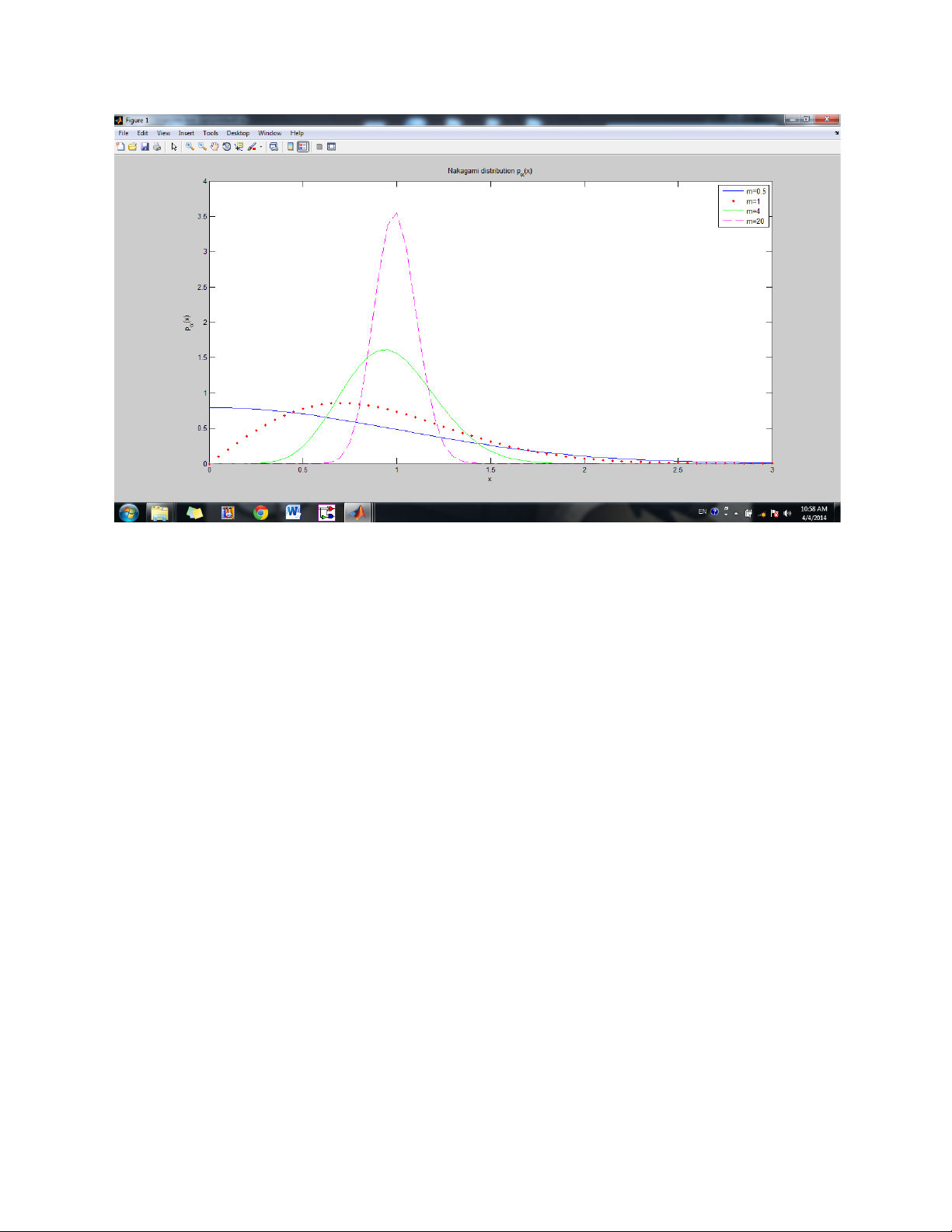
% ================================== % Nakagami distribution
% ================================== clear;
m1=0.5; % The Nakagami shape factor m2=1; m3=4; m4=20; ohm_p=1; x=0:0.05:3; m=m1;
p_alpha1=(2*m^m.*x.^(2*m-1)/gamma(m)*ohm_p^m).*exp(-m.*x.^2/ohm_p); plot(x,p_alpha1) hold on m=m2;
p_alpha2=(2*m^m.*x.^(2*m-1)/gamma(m)*ohm_p^m).*exp(-m.*x.^2/ohm_p); plot(x,p_alpha2,'r.') m=m3;
p_alpha3=(2*m^m.*x.^(2*m-1)/gamma(m)*ohm_p^m).*exp(-m.*x.^2/ohm_p); plot(x,p_alpha3,'g-') m=m4;
p_alpha4=(2*m^m.*x.^(2*m-1)/gamma(m)*ohm_p^m).*exp(-m.*x.^2/ohm_p); plot(x,p_alpha4,'m--') hold off
title('Nakagami distribution p_{\alpha}(x)') xlabel('x') ylabel('p_{\alpha}(x)')
legend('m=0.5','m=1','m=4','m=20') Exercise 3.3.2
% =====================================================
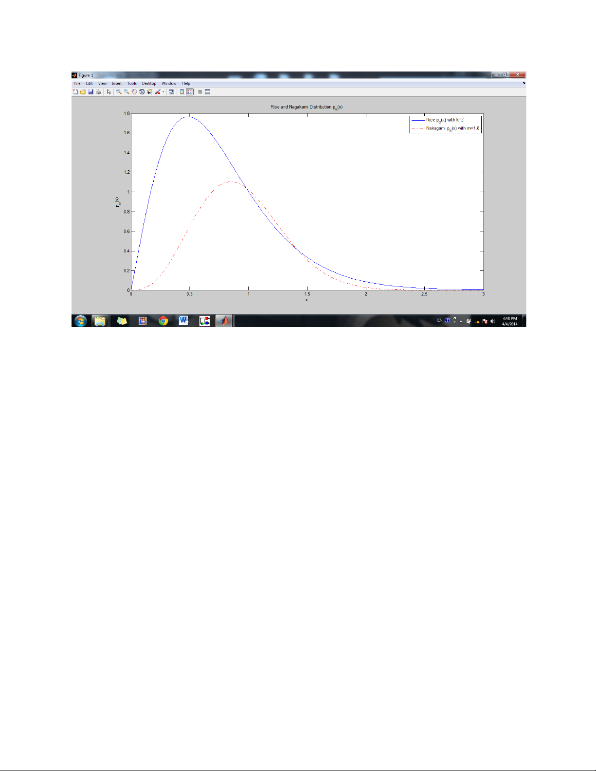
% The Rice and Nagakami distribution
% ===================================================== clear;
k=2; % the rice factor k=s^2/2b_0
x=0:0.01:3; % the time interval in seconds
ohm_p=1; % the total received power
p_elfa=(2.*x.*(k+1)/ohm_p).*exp(((-k-(k+1)).*x./ohm_p)).*besseli(0,(2*sqrt(k*(k +1).*x./ohm_p))); plot(x,p_elfa) hold on m=1.8;
p_alpha1=(2*m^m.*x.^(2*m-1)/gamma(m)*ohm_p^m).*exp(-m.*x.^2/ohm_p); plot(x,p_alpha1,'r-.') hold off
title('Rice and Nagakami Distribution p_{\alpha}(x)') xlabel('x') ylabel('p_{\alpha}(x)')
legend('Rice p_{\alpha}(x) with k=2','Nakagami p_{\alpha}(x) with m=1.8') Exercise 4.1
% ==============================================
% Calculation of simulation parameters
% ============================================== clear;
f_m=91; % Maximal Doppler frequency
b=1; % Variance of in-phase or quadrature component
N1=9; % Number of sinusoids for the in-phase component
N2=10; % Number of sinusoids for the quadrature component for n=1:1:N1; c1(n)=sqrt(2*b/N1);
f1(n)=f_m*sin(pi*(n-0.5)/(2*N1)); th1(n)=2*pi*n/(N1+1); end for n=1:1:N2; c2(n)=sqrt(2*b/N2);
f2(n)=f_m*sin(pi*(n-0.5)/(2*N2)); th2(n)=2*pi*n/(N2+1); end
save ex4p1_Res f1 f2 c1 c2 th1 th2
% these result will be use in the exercise 4.3 and 4.4 Exercise 4.2
% ===================================================
% a function which creates the determisistic process g(t)
% save this function to a file name "g.m"
% =================================================== function y=g(c,f,th,t) y=zeros(site(t)); for n=1:length(f);
y=y+c(n)*cos(2*pi*f(n).*t+th(n)); end Exercise 4.3
% ===========================================
% Crate a deterministic process by Rice method
% =========================================== clear;
load ex4p1_Res f1 f2 c1 c2 th1 th2
f_s = 270800; % the carrier frequency in Hz
T_sim = 0.4; % Simulation time in second
t = 0:1/f_s:T_sim; % discrete time interval
g1 = g(c1, f1, th1, t); % generation of the process g1 by using the function "g.m" from the excercise 4.2 g2 = g(c2, f2, th2, t); g = g1+j*g2; alpha = abs(g); alpha_dB = 20*log10(alpha); plot(t, alpha_dB);
title('The channel amplitude in dB'); xlabel('t'); ylabel('\alpha(t)'); legend('\alpha(t) in dB', 0); Exercise 4.4
% =========================================================
% Comparision of theoretical Gaussian and Reyleigh distribution with % simulations results
% ========================================================= clear;
load ex4p1_Res f1 f2 c1 c2 th1 th2
f_s = 50000; % the carrier frequency in Hz
T_sim = 20; % simulation time in seconds t = 0:1/f_s:T_sim; g1 = g(c1, f1, th1, t); g2 = g(c2, f2, th2, t); g = g1+j*g2; alpha = abs(g); g_mean = mean(g); g_variance = var(g); g1_mean = mean(g1); g1_variance = var(g1); alpha_mean = mean(alpha); alpha_variance = var(alpha); n = length(alpha);
x = 0:0.1:3; % the time interval in seconds b = hist(alpha, x); figure(1); stem(x, b/n/(x(2)-x(1))); hold on;
k = 0; % the rice factor k=s^2/2b_0
ohm_p = 2; % the total received power
p_alpha = (2*x*(k+1)/ohm_p).*exp(-k-((k+1)*x.^2/ohm_p)).*besseli(0, (2*x.*sqrt(k*(k+1)/ohm_p))); plot(x, p_alpha, 'r');
title('The PDF of {\alpha}(x)'); xlabel('x'); ylabel('P_{\alpha}(x)');
legend('p_{\alpha}(x)', 'Rayleigh distribution (Theory)'); hold off; figure(2); n1 = length(g1); x1 = -4:0.1:4; c = hist(g1, x1); stem(x1, c/n1/(x1(2)-x1(1))); hold on;
p = (1/sqrt(2*pi))*exp(-x1.^2/2); plot(x1, p, 'r');
title('The PDF of g1 process'); xlabel('x'); ylabel('P_{g1}(x)');
legend('p_{g1}(x)', 'Gaussian distribution (Theory)'); hold off; Exercise 4.5
% =============================================================
% Autocorrelation result of g1 process
% ============================================================= clear;
load ex4p1_Res f1 f2 c1 c2 th1 th2
f_s = 1000; % the carrier frequency in Hz
T_s = 1/f_s; % the sampling time in seconds I1 = 10000*T_s; I2 = 20000*T_s; t = I1:T_s:I2; g1 = g(c1, f1, th1, t);
phi_g1g1 = xcorr(g1, 'biased'); i = 1:81; x = (i-1)*T_s;
phi_g1g1_select = phi_g1g1(10001:10081); plot(x, phi_g1g1_select);
title('The autocorrelation function ACF of g1'); xlabel('\tau in seconds'); ylabel('\phi_{g1g1}(\tau)');
legend('\phi_{g1g1}(\tau) of g1');
save ex4p5_Res phi_g1g1_select f_s phi_g1g1; Exercise 4.6
% ========================================================
% Simulation result of ACF of g1 in comparison with theoretical result
% ======================================================== clear;
f_m = 91; % Maximum Doppler frequency b = 1; N1 = 9; % Number of sinusoids tau_max = 0.08;
t_a = 0.001; % Sampling interval for n = 1:N1 c1(n) = sqrt(2*b/N1);
f1(n) = f_m*sin(pi*(n-0.5)/(2*N1)); th1(n) = 2*pi*n/(N1+1); end tau = 0:t_a:tau_max; k = 1:length(tau); for n = 1:N1
x(n, k) = (c1(n).^2/2)*cos(2*pi*f1(n).*tau); end fay = sum(x); tau_s = -tau_max:t_a:tau_max; k = 1:length(tau_s); for n = 1:N1
xs(n, k) = (c1(n).^2/2)*cos(2*pi*f1(n).*tau_s); end phi_g1g1_theory = sum(xs); plot(tau, fay); hold on;
f_c = 900e6; % The carrier frequency in Hz c_0 = 3e8; % The speed of light in m/s
v = 109.2e3/3600; % The mobile station's speed in m/s f_m = v*f_c/c_0;
% The maximum doppler frequency ohm_p = 2; % The total received power t = 0:0.001:tau_max; z = 2*pi*f_m*t;
phi_g1g1 = (ohm_p/2)*besselj(0, z); % The autocorrelation function plot(tau, phi_g1g1, 'r'); load ex4p5_Res; N = length(phi_g1g1);
phi_g1g1_s = phi_g1g1(N/2:N/2+tau_max/t_a); plot(tau, phi_g1g1_s, 'k');
title('The autocorrelation function (ACF) of the process g1'); xlabel('\tau in seconds'); ylabel('\phi_{g1g1}(\tau)');
legend('\phi_{g1g1}(\tau) Simulation model (Theory)',