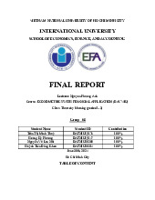
Bài tập tiểu luận nhóm học phần Econometrics with Financial Application | Trường Đại học Quốc tế, Đại học Quốc gia Thành phố Hồ Chí Minh

International University – HCMC
Econometrics with Financial Application
Vietnam National University – HCMC
International University – HCMC
Econometrics with Financial Application International University HOMEWORK CHAPTER 6 SCHOOL OF BUSINESS Question 1:
You obtain the following sample autocorrelations and partial autocorrelations for a sample of
100 observations from actual data: Lag 1 2 3 4 5 6 7 8 ACF 0.420 0.104 0.032 -0.206 -0.138 0.042 -0.018 0.074 PACF 0.632 0.381 0.268 0.199 0.205 0.101 0.096 0.082
Can you identify the most appropriate time series process for this data?
Using the Ljung-Box Q* test to determine whether the first three autocorrelation coefficients
taken together are jointly significantly different from zero. Answer: Single test: 𝐻 :𝜏 = 0
Econometrics with Financial Application_S2_2022-23_G01 Dr Using confidential interval Nguyen Phuong Anh
0.42 > 0.196 => Reject 𝐻 :𝜏 = 0
-0.196 < 0.104 < 0.196 => Not reject 𝐻 :𝜏 = 0
-0.196 < 0.032 < 0.196 => Not reject 𝐻 :𝜏 = 0
-0.206 < 0.196 => Reject 𝐻 : 𝜏 = 0 Seq. Full name Student ID Contribution
-0.196 < -0.138 < 0.196 => Not reject 𝐻 : 𝜏 = 0 1 Trương Phúc An BABAIU20526 100%
-0.196 < 0.042 < 0.196 => Not reject 𝐻 :𝜏 = 0
-0.196 < -0.018 < 0.196 => Not reject 𝐻 : 𝜏 = 0 2 Nguyễn Hoàng Bảo Hân BAFNIU19077 100%
-0.196 < 0.074 < 0.196 => Not reject 𝐻 :𝜏 = 0
Since only 𝜏 ≠ 0 𝑎𝑛𝑑 𝜏
≠ 0 => 𝐴𝐶𝐹 = 0 𝑎𝑓𝑡𝑒𝑟 4 𝑙𝑎𝑔𝑠 3 Hồ Thế Phong BAFNIU19141 100% |𝜏 | = 0.643 |𝜏 | = 0.381 |𝜏 | = 0.268 Page 1 of 5
This shows that PACF is slowly decaying to 0
International University – HCMC
Econometrics with Financial Application Page 2 of 5 0.68
→ 𝐴𝑅𝑀𝐴 𝑖𝑠 𝑖𝑛𝑣𝑒𝑟𝑡𝑖𝑏𝑙𝑒
• MA is more suitable. Since ACF = 0 after 4 lags, we use MA (4). Page 3 of 5 Ljung-box formula: 𝐻 : 𝜏 = 𝜏 = 𝜏 = 0 (𝑚 = 3)
International University – HCMC
Econometrics with Financial Application
• Test statistic Q* compared with CV from 2 (3) • Question 3: CV=7.815 •
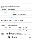
Considering the following 3 models that a researcher suggests might be a reasonable model of
𝑄∗ = 𝑇 × (𝑇 + 2) ∑ stock market prices:
• 𝑄∗ = 19.4 > 𝐶𝑉 => 𝑄∗ 𝑏𝑒𝑙𝑜𝑛𝑔𝑠 𝑡𝑜 𝑡ℎ𝑒 𝑟𝑒𝑗𝑒𝑐𝑡𝑖𝑜𝑛 𝑟𝑒𝑔𝑖𝑜𝑛 i) 𝑦 = 0.7𝑢 + 𝑢
• 𝑅𝑒𝑗𝑒𝑐𝑡 𝐻 : 𝜏 = 𝜏 = 𝜏 = 0 j) 𝑦 = 0.4𝑦 + 𝑢
• The first three autocorrelation coefficients taken together are jointly k) 𝑦 = 2𝑦 + 𝑢
significantly different from zero Question 2:
a) What classes of model are these examples of?
b) Are these models stationary?
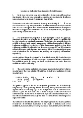
Considering the following ARMA process:
c) Calculate the autocorrelation coefficients for the process (i) and (j) up to lag 2. 𝑦 = 2.1 + 1.5𝑦 + 0.68𝑢 + 𝑢 Answer:
Determine whether the MA part of the process is invertible.
a) i is MA. While j and k is AR.
Determine whether the AR part of the process is stationary.
b) Since MA is always stationary => i is stationary 𝑗) 𝑦 = 0.4𝑦 + 𝑢 Answer:
↔ 𝑦 = 0.4𝐿𝑦 + 𝑢 (1 −
ARMA (1, 1) model is stationary when AR part is stationary 0.4𝐿)𝑦 = 𝑢 𝑦 = 2.1 + 1.5𝑦 (𝐴𝑅(1))
𝛷(𝑍) = 0 ↔ 1 − 0.4𝑍 = 0 𝑦 − 1.5𝑦 = 2.1 + 0.68𝑢 + 𝑢 1
𝑦 − 1.5𝐿𝑦 = 2.1 + 0.68𝐿𝑢 + 𝑢 → 𝑍 =
> 1 → 𝑜𝑢𝑡𝑠𝑖𝑑𝑒 𝑢𝑛𝑖𝑡 𝑐𝑖𝑟𝑐𝑙𝑒 → 𝑆𝑡𝑎𝑡𝑖𝑜𝑛𝑎𝑟𝑦
(1 − 1.5𝐿)𝑦 = 2.1 + (0.68𝐿 + 1)𝑢 0.4 𝑘) 𝑦 = 2𝑦 + 𝑢
(1 − 1.5𝐿)𝑦 = 𝛷(𝐿), (0.68𝐿 + 1)𝑢 = 𝜃(𝐿)
↔ 𝑦 = 2𝐿𝑦 + 𝑢 (1 −
𝛷(𝑍) = 0 ↔ 1 − 1.5𝑍 = 0 2𝐿)𝑦 = 𝑢 1 → 𝑍 =
< 1 → 𝑖𝑛𝑠𝑖𝑑𝑒 𝑢𝑛𝑖𝑡 𝑐𝑖𝑟𝑐𝑙𝑒 → 𝐴𝑅 𝑝𝑎𝑟𝑡 𝑖𝑠 𝑛𝑜𝑡 𝑠𝑡𝑎𝑡𝑖𝑜𝑛𝑎𝑟𝑦
𝛷(𝑍) = 0 ↔ 1 − 2𝑍 = 0 1.5
𝜃(𝐿) = 0 ↔ 0.68𝑍 + 1 = 0
→ 𝑍 = < 1 → 𝑖𝑛𝑠𝑖𝑑𝑒 𝑢𝑛𝑖𝑡 𝑐𝑖𝑟𝑐𝑙𝑒 → 𝑁𝑜𝑡 𝑠𝑡𝑎𝑡𝑖𝑜𝑛𝑎𝑟𝑦 1 → |𝑍| =
> 1 → 𝑜𝑢𝑡𝑠𝑖𝑑𝑒 𝑢𝑛𝑖𝑡 𝑐𝑖𝑟𝑐𝑙𝑒 → 𝑀𝐴 𝑝𝑎𝑟𝑡 𝑖𝑠 𝑖𝑛𝑣𝑒𝑟𝑡𝑖𝑏𝑙𝑒
International University – HCMC
Econometrics with Financial Application
c) 𝐴𝑅(1): 𝑦 = 0.4𝑦 + 𝑢 + 0 × 𝑦 Yule-Walker system 𝜏 = 𝛷 + 𝜏 × 0 = 0.4 i) 𝑦 = 0.7𝑢 + 𝑢 𝑀𝐴(1) 𝛾
𝜏 = , 𝛾 = 𝑉𝑎𝑟(𝑦 ) 𝛾
(𝑖) → 𝐸(𝑦 ) = 𝐸(0.7𝑢 + 𝑢 ) Page 4 of 5 Page 5 of 5
= 0.7𝐸(𝑢 ) + 𝐸(𝑢 )
(𝑖) → 𝑉𝑎𝑟(𝑦 ) = 𝐶𝑜𝑣(𝑦 , 𝑦 )
= 𝐸[(𝑦 − 0)(𝑦 − 0)] = 𝐸[(0.7𝑢 + 𝑢 )(0.7𝑢 + 𝑢 )] = 𝐸[(0.7 𝑢 + 𝑢 + 1.4𝑢 𝑢 )] = (0.7 + 1)𝑉𝑎𝑟𝑢 = (0.7 + 1)𝜎 𝑢
(𝑖) → 𝛾 = 𝐶𝑜𝑣(𝑦 , 𝑦 ) = 𝐸[(𝑦 − 0)(𝑦 − 0)] = 𝐸[(0.7𝑢 + 𝑢 )(0.7𝑢 + 𝑢 )] = 𝐸[(0.7 𝑢 𝑢 + 𝑢 𝑢 + 1.4𝑢 )] = 1.4𝜎 𝑢 . . Then 𝜏 = =
Similarly, 𝜏 = = 𝐶𝑜𝑣 𝑦 ,𝑦 = =0 𝑉𝑎𝑟 𝑦𝑡
For MA (1), ACF = 0 after q lags.