Vietnam National University – HCMC CAPM International University SCHOOL OF BUSINESS
The term "sum of squares" or "SS" is used to denote variation. The target variable's
variance is made up of the model's (explainable variance) and the residuals' (unexplainable
variance) variances. The target variable's entire variation from its mean is what is meant
by the term total SS. From the output, we can see that out of a variation of 34,741.3443 in
the dependent variable, 11,721.7394 is explainable by the model, while the remaining 23,019.605 is unexplainable.
Econometrics with Financial Application_S2_2022-
The degree of freedom (df) connected to a variance is called df. The number of
independently variable values is referred to as the degree of freedom. The output shows 23_G01
that the residuals and model degrees of freedom are 1 and 191 respectively, while the
overall degree of freedom is 192. Dr Nguyen Phuong Anh
The square root of the mean value is ms. It is the sum of squares divided by the degree of
freedom, or the sum of squares per unit of freedom. The mean sum of squares for the
model, residual, and total are, according to the output, 11,721.7394, 120.521492, and 180.944502, respectively. Seq. Full name Student ID Contribution
Number of obs is simply the number of observations used in the regression. Since the data
has 193 observations, Number of obs is equal to 193. 1 Trương Phúc An BABAIU20526 100%
F(1, 191) is the F-statistics of an ANOVA test run on the model. The F-statistics is the ratio
of the mean sum of squares (ms) of the model to that of the residual. It measures how the 2 Nguyễn Hoàng Bảo Hân BAFNIU19077 100%
ratio of the explainable mean variance to the unexplainable mean variance is statistically
greater than 1. The 1 and 192 simply represents the model’s and residual degrees of 3
freedom respectively. To know how well the predictors (taken together as a group) reliably Hồ Thế Phong BAFNIU19141 100%
predicts the dependent variable, Stata conducts a hypothesis test using the F-statistics. Homework
The null hypothesis is that the mean explainable variance is same as the mean unexplainable variance.
The Prob > F is the probability of obtaining the estimated F-statistics or greater (the
pvalue). For a typical alpha level of 0.05, a p-value lesser than 0.05 like we have in
our output, means that we have evidence to reject the null hypothesis and accept
the alternate hypothesis that the ms of the model is significantly greater than that
of the residual. Hence, the predictors of our model reliably predict the target variable.
R-squared is the coefficient of determinant and it represents the goodness of fit. It
is numerically the fraction of the variation in the dependent variable that can be
accounted for (explained) by the independent variables. From the output, 33.74%
of the variation in the dependent variable are explainable by the model.
Adj R-squared: Since the addition of more and more predictors tend to increase the
The term "sum of squares" or "SS" is used to denote variation. The target variable's
Rsquared, Adj R-squared tells us how much of the variation of the dependent
variance is made up of the model's (explainable variance) and the residuals' (unexplainable
variable is determined by the addition of the independent variables. Adj R-squared
variance) variances. The target variable's entire variation from its mean is what is meant
is the R-squared controlled for by the number of predictors. From the output, we
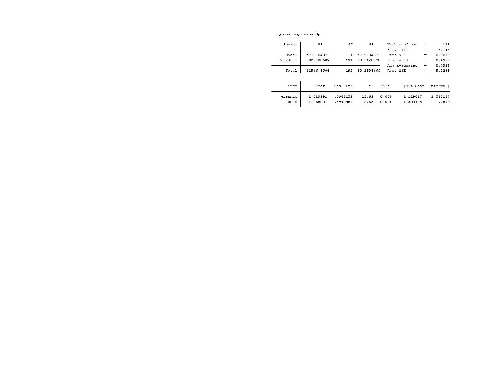
by the term total SS. From the output, we can see that out of a variation of 11,546.8506 in
can say that after adjusting for the degree of freedom, the coefficient of the
the dependent variable, 5,719.04373 is explainable by the model, while the remaining determinant is 33.39% 11,546.8506 is unexplainable.
Root MSE is simply the standard deviation of the residuals (error term). From the
The degree of freedom (df) connected to a variance is called df. The number of
output, we can say that the measure of the spread of the residuals is 10.978
independently variable values is referred to as the degree of freedom. The output shows
that the residuals and model degrees of freedom are 1 and 191 respectively, while the
The beta coefficient (the slope coefficient) estimate is 1.89 with a t-ratio of 9.86 and
overall degree of freedom is 192.
a corresponding p-value of 0.000. This suggests that the excess return on the market
proxy has highly significant explanatory power for the variability of the excess return
The square root of the mean value is ms. It is the sum of squares divided by the degree of of Ford stock.
freedom, or the sum of squares per unit of freedom. The mean sum of squares for the
model, residual, and total are, according to the output, 5,719.04373, 30.5120778, and
Let us turn to the intercept now. The α estimate is –0.96 with a t-ratio of –1.21 and 60.1398469, respectively.
a pvalue of 0.230. Thus, we cannot reject that the α estimate is different from 0,
indicating that the Ford stock does not seem to significantly outperform or
Number of obs is simply the number of observations used in the regression. Since the data
underperform the overall market.
has 193 observations, Number of obs is equal to 193.
F(1, 191) is the F-statistics of an ANOVA test run on the model. The F-statistics is the ratio
of the mean sum of squares (ms) of the model to that of the residual. It measures how the
ratio of the explainable mean variance to the unexplainable mean variance is statistically
greater than 1. The 1 and 192 simply represents the model’s and residual degrees of
freedom respectively. To know how well the predictors (taken together as a group) reliably
predicts the dependent variable, Stata conducts a hypothesis test using the F-statistics.
The null hypothesis is that the mean explainable variance is same as the mean unexplainable variance.
The Prob > F is the probability of obtaining the estimated F-statistics or greater (the
pvalue). For a typical alpha level of 0.05, a p-value lesser than 0.05 like we have in
our output, means that we have evidence to reject the null hypothesis and accept
the alternate hypothesis that the ms of the model is significantly greater than that
of the residual. Hence, the predictors of our model reliably predict the target variable.
R-squared is the coefficient of determinant and it represents the goodness of fit. It
is numerically the fraction of the variation in the dependent variable that can be
accounted for (explained) by the independent variables. From the output, 49.53%
of the variation in the dependent variable are explainable by the model.
Adj R-squared: Since the addition of more and more predictors tend to increase the
Rsquared, Adj R-squared tells us how much of the variation of the dependent
variable is determined by the addition of the independent variables. Adj R-squared
The term "sum of squares" or "SS" is used to denote variation. The target variable's
is the R-squared controlled for by the number of predictors. From the output, we
variance is made up of the model's (explainable variance) and the residuals' (unexplainable
can say that after adjusting for the degree of freedom, the coefficient of the
variance) variances. The target variable's entire variation from its mean is what is meant determinant is 49.26%
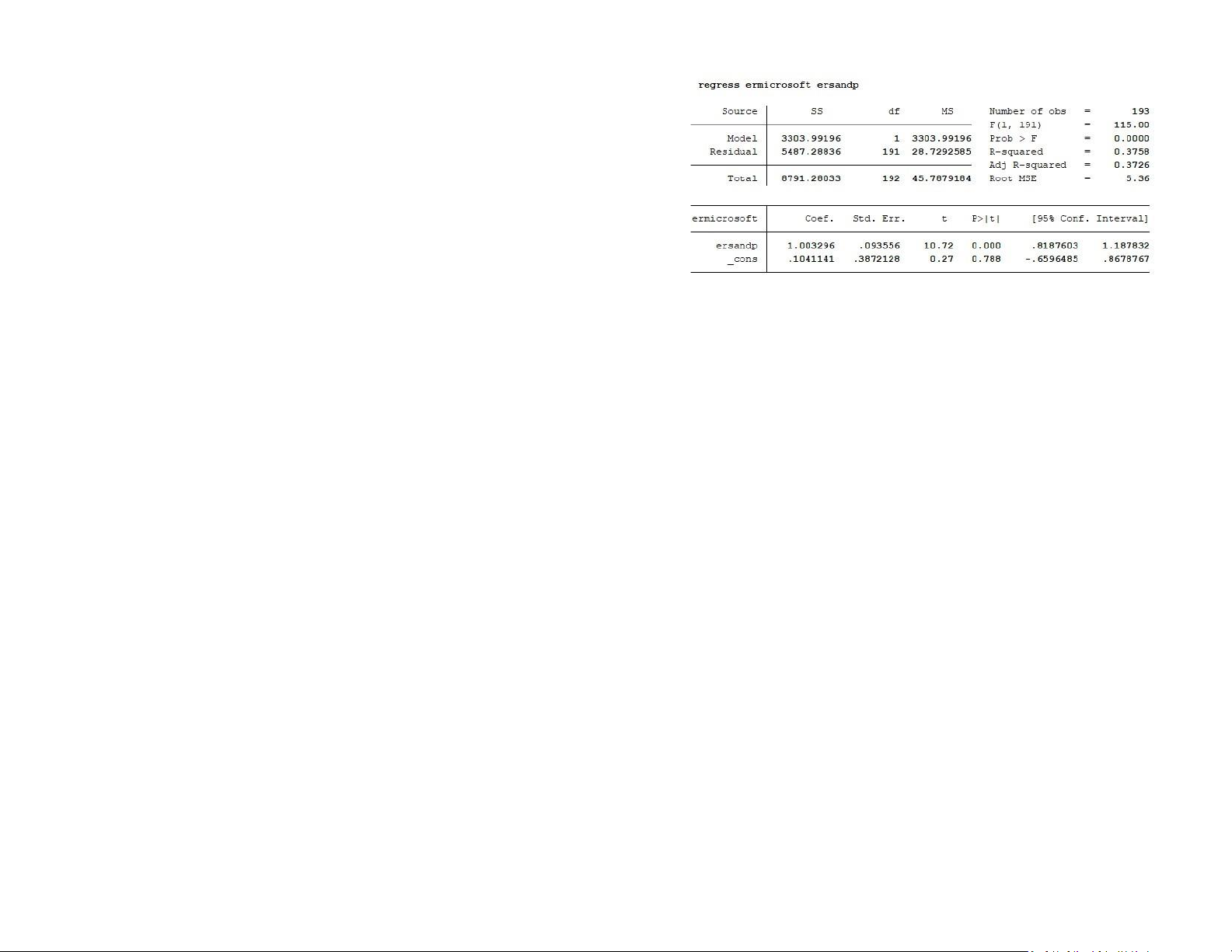
by the term total SS. From the output, we can see that out of a variation of 8,791.28033 in
Root MSE is simply the standard deviation of the residuals (error term). From the
the dependent variable, 3,303.99196 is explainable by the model, while the remaining
output, we can say that the measure of the spread of the residuals is 5.5238 5,487.28836 is unexplainable.
The beta coefficient (the slope coefficient) estimate is 1.32 with a t-ratio of 13.69
The degree of freedom (df) connected to a variance is called df. The number of
and a corresponding p-value of 0.000. This suggests that the excess return on the
independently variable values is referred to as the degree of freedom. The output shows
market proxy has highly significant explanatory power for the variability of the
that the residuals and model degrees of freedom are 1 and 191 respectively, while the excess return of GE stock.
overall degree of freedom is 192.
Let us turn to the intercept now. The α estimate is –1.07 with a t-ratio of –2.68 and
The square root of the mean value is ms. It is the sum of squares divided by the degree of
a pvalue of 0.008. Thus, indicating that the GE stock has significantly underperform
freedom, or the sum of squares per unit of freedom. The mean sum of squares for the the overall market.
model, residual, and total are, according to the output, 3,303.99196, 28.7292585, and 45.7879184, respectively.
Number of obs is simply the number of observations used in the regression. Since the data
has 193 observations, Number of obs is equal to 193.
F(1, 191) is the F-statistics of an ANOVA test run on the model. The F-statistics is the ratio
of the mean sum of squares (ms) of the model to that of the residual. It measures how the
ratio of the explainable mean variance to the unexplainable mean variance is statistically
greater than 1. The 1 and 192 simply represents the model’s and residual degrees of
freedom respectively. To know how well the predictors (taken together as a group) reliably
predicts the dependent variable, Stata conducts a hypothesis test using the F-statistics.
The null hypothesis is that the mean explainable variance is same as the mean unexplainable variance.
The Prob > F is the probability of obtaining the estimated F-statistics or greater (the
pvalue). For a typical alpha level of 0.05, a p-value lesser than 0.05 like we have in
our output, means that we have evidence to reject the null hypothesis and accept
the alternate hypothesis that the ms of the model is significantly greater than that
of the residual. Hence, the predictors of our model reliably predict the target variable.
R-squared is the coefficient of determinant and it represents the goodness of fit. It
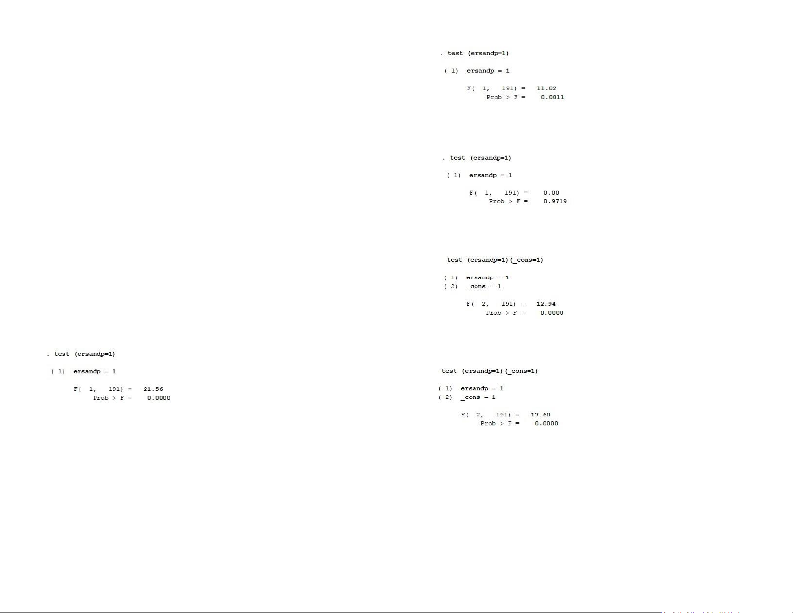
The F-statistic of 11.02 with a corresponding p-value of 0.0011 implying that the null
is numerically the fraction of the variation in the dependent variable that can be
hypothesis that the CAPM beta of GE stock is 1 is convincingly rejected and hence the
accounted for (explained) by the independent variables. From the output, 37.58%
estimated beta of 1.32 is significantly different from 1.31
of the variation in the dependent variable are explainable by the model.
Adj R-squared: Since the addition of more and more predictors tend to increase the
Rsquared, Adj R-squared tells us how much of the variation of the dependent
variable is determined by the addition of the independent variables. Adj R-squared
is the R-squared controlled for by the number of predictors. From the output, we
can say that after adjusting for the degree of freedom, the coefficient of the determinant is 37.26%
The F-statistic of 0 with a corresponding p-value of 0.9719 implying that the null hypothesis
Root MSE is simply the standard deviation of the residuals (error term). From the
that the CAPM beta of Microsoft stock is 1 is convincingly not rejected and hence the
output, we can say that the measure of the spread of the residuals is 5.36
estimated beta of 1 is not different from 1
The beta coefficient (the slope coefficient) estimate is 1 with a t-ratio of 10.72 and a
corresponding p-value of 0.000. This suggests that the excess return on the market
proxy has highly significant explanatory power for the variability of the excess return of Microsoft stock.
Let us turn to the intercept now. The α estimate is 0.104 with a t-ratio of 0.27 and a
p-value of 0.788. Thus, we cannot reject that the α estimate is different from 0,
indicating that the Microsoft stock does not seem to significantly outperform or
Looking at the value of the F-statistic of 12.94 with a corresponding p-value of 0.0000, we
underperform the overall market.
conclude that the null hypothesis, H0: β1 = 1 and β2 = 1, is strongly rejected at the 1% significance level.
The F-statistic of 21.56 with a corresponding p-value of 0 (at least up to the fourth
decimal point) implying that the null hypothesis that the CAPM beta of Ford stock is
1 is convincingly rejected and hence the estimated beta of 1.89 is significantly different from 1.
Looking at the value of the F-statistic of 17.6 with a corresponding p-value of 0.0000,
The degree of freedom (df) connected to a variance is called df. The number of
we conclude that the null hypothesis, H0: β1 = 1 and β2 = 1, is strongly rejected at
independently variable values is referred to as the degree of freedom. The output shows the 1% significance level.
that the residuals and model degrees of freedom are 7 and 375 respectively, while the
overall degree of freedom is 382.
The square root of the mean value is ms. It is the sum of squares divided by the degree of
freedom, or the sum of squares per unit of freedom. The mean sum of squares for the
model, residual, and total are, according to the output, 1,738.09797, 61.5416232, and 92.26386, respectively.
Number of obs is simply the number of observations used in the regression. Since the data
has 383 observations, Number of obs is equal to 383.
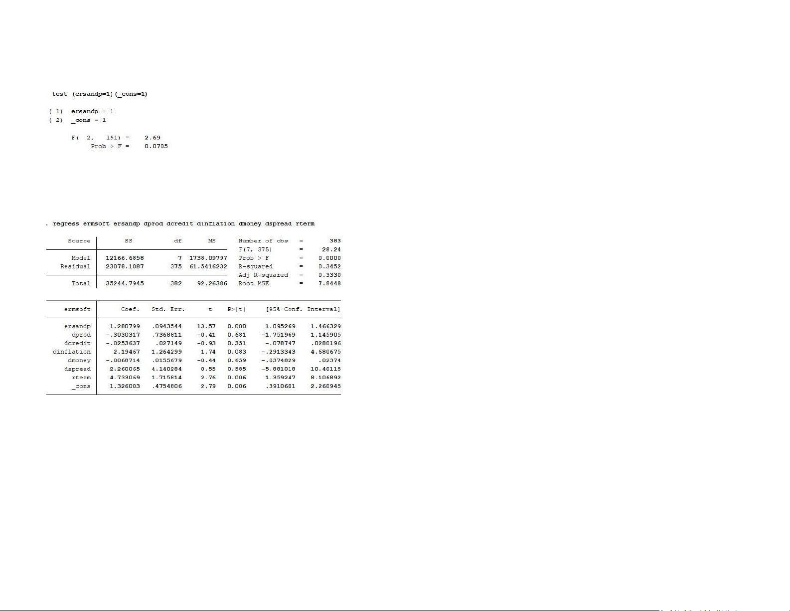
Looking at the value of the F-statistic of 2.69 with a corresponding p-value of 0.0705,
we conclude that the null hypothesis, H0: β1 = 1 and β2 = 1, is not rejected at the
F (7, 375) is the F-statistics of an ANOVA test run on the model. The F-statistics is the ratio 1% significance level.
of the mean sum of squares (ms) of the model to that of the residual. It measures how the
ratio of the explainable mean variance to the unexplainable mean variance is statistically Macro
greater than 1. The 7 and 375 simply represents the model’s and residual degrees of
freedom respectively. To know how well the predictors (taken together as a group) reliably
predicts the dependent variable, Stata conducts a hypothesis test using the F-statistics.
The null hypothesis is that the mean explainable variance is same as the mean unexplainable variance.
The Prob > F is the probability of obtaining the estimated F-statistics or greater (the pvalue).
For a typical alpha level of 0.05, a p-value lesser than 0.05 like we have in our output,
means that we have evidence to reject the null hypothesis and accept the alternate
hypothesis that the ms of the model is significantly greater than that of the residual. Hence,
the predictors of our model reliably predict the target variable.
R-squared is the coefficient of determinant and it represents the goodness of fit. It is
numerically the fraction of the variation in the dependent variable that can be accounted
for (explained) by the independent variables. From the output, 34.52% of the variation in
the dependent variable are explainable by the model.
Adj R-squared: Since the addition of more and more predictors tend to increase the
Rsquared, Adj R-squared tells us how much of the variation of the dependent variable is
determined by the addition of the independent variables. Adj R-squared is the R-squared
controlled for by the number of predictors. From the output, we can say that after
The term "sum of squares" or "SS" is used to denote variation. The target variable's
adjusting for the degree of freedom, the coefficient of the determinant is 33.3%
variance is made up of the model's (explainable variance) and the residuals'
Root MSE is simply the standard deviation of the residuals (error term). From the output,
(unexplainable variance) variances. The target variable's entire variation from its
we can say that the measure of the spread of the residuals is 7.8448
mean is what is meant by the term total SS. From the output, we can see that out
of a variation of 35,244.7945 in the dependent variable, 12,166.6858 is explainable
The beta coefficient (the slope coefficient) estimate with corresponding p-value of 0.000
by the model, while the remaining 23,078.1087 is unexplainable.
or less than 0.05. This suggests that the excess return on the market proxy has highly
significant explanatory power for the variability of ersandp, rterm. However, there
shows that the residuals and model degrees of freedom are 3 and 379 respectively, while
are no significant explanatory for dprod, dcredit, dinflation, dmoney, and dspread.
the overall degree of freedom is 382.
Let us turn to the intercept now. The α estimate is 1.33 with a t-ratio of 2.79 and a
The square root of the mean value is ms. It is the sum of squares divided by the degree of
p-value of 0.006. Thus, Thus, indicating that the Microsoft stock has significantly
freedom, or the sum of squares per unit of freedom. The mean sum of squares for the
overperform the overall market.
model, residual, and total are, according to the output, 4,021.60092, 61.1609281, and 92.26386, respectively.
Number of obs is simply the number of observations used in the regression. Since the data
has 383 observations, Number of obs is equal to 383.
F (7, 375) is the F-statistics of an ANOVA test run on the model. The F-statistics is the ratio
of the mean sum of squares (ms) of the model to that of the residual. It measures how the
ratio of the explainable mean variance to the unexplainable mean variance is statistically
greater than 1. The 3 and 379 simply represents the model’s and residual degrees of
freedom respectively. To know how well the predictors (taken together as a group) reliably
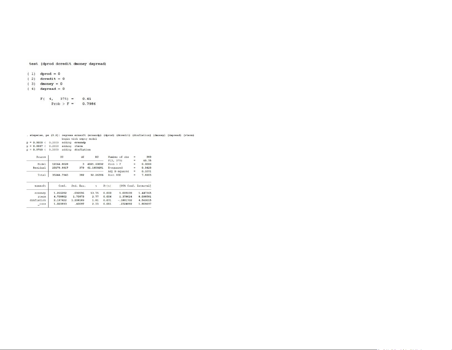
The F-statistic value is 0.41 with p-value 0.7986, suggesting that the null hypothesis
predicts the dependent variable, Stata conducts a hypothesis test using the F-statistics.
cannot be rejected. The parameters on ‘rterm’ and ‘dinflation’ are significant at the
The null hypothesis is that the mean explainable variance is same as the mean
10% level. Hence, they are not included in this F-test and the variables are retained. unexplainable variance.
The Prob > F is the probability of obtaining the estimated F-statistics or greater (the pvalue).
For a typical alpha level of 0.05, a p-value lesser than 0.05 like we have in our output,
means that we have evidence to reject the null hypothesis and accept the alternate
hypothesis that the ms of the model is significantly greater than that of the residual. Hence,
the predictors of our model reliably predict the target variable.
R-squared is the coefficient of determinant and it represents the goodness of fit. It is
numerically the fraction of the variation in the dependent variable that can be accounted
for (explained) by the independent variables. From the output, 34.23% of the variation in
the dependent variable are explainable by the model.
Adj R-squared: Since the addition of more and more predictors tend to increase the
Rsquared, Adj R-squared tells us how much of the variation of the dependent variable is
determined by the addition of the independent variables. Adj R-squared is the R-squared
The term "sum of squares" or "SS" is used to denote variation. The target variable's
controlled for by the number of predictors. From the output, we can say that after
variance is made up of the model's (explainable variance) and the residuals'
adjusting for the degree of freedom, the coefficient of the determinant is 33.71%
(unexplainable variance) variances. The target variable's entire variation from its
mean is what is meant by the term total SS. From the output, we can see that out
Root MSE is simply the standard deviation of the residuals (error term). From the output,
of a variation of 35,244.7945 in the dependent variable, 12,064.8028 is explainable
we can say that the measure of the spread of the residuals is 7.8205
by the model, while the remaining 23,179.9917 is unexplainable.
The beta coefficient (the slope coefficient) estimate with corresponding p-value of 0.000
The degree of freedom (df) connected to a variance is called df. The number of
or less than 0.2. This suggests that the excess return on the market proxy has highly
independently variable values is referred to as the degree of freedom. The output
significant explanatory power for the variability of ersandp, rterm, dinflation. If any other
variable is in the 20% significant or higher, we should add that variable.
Let us turn to the intercept now. The α estimate is 1.02 with a t-ratio of 2.55 and a
p-value of 0.011. Thus, Thus, indicating that the Microsoft stock has slightly
overperform the overall market.