Báo cáo thí nghiệm RLC C1: Đo Đạc Trở, Tụ và Tần Số Resonance môn Vật lý đại cương 2 | Trường Đại học Bách Khoa Hà Nội

HANOI UNIVERSITY OF SCIENCE AND TECHNOLOGY
SCHOOL OF ENGINEERING PHYSICS Physics 2
Experimental Report
Full name: Nguyn Văn Nhâ t Student ID: 20237035 Class: 746179 Group: 05 1 Experimental Report 1
MEASUREMENT OF RESISTANCE, CAPACITANCE,
INDUCTANCE AND RESONANT FREQUENCIES OF RLC
CIRCUIT USING OSCILLOSCOPE I. Data Tables:
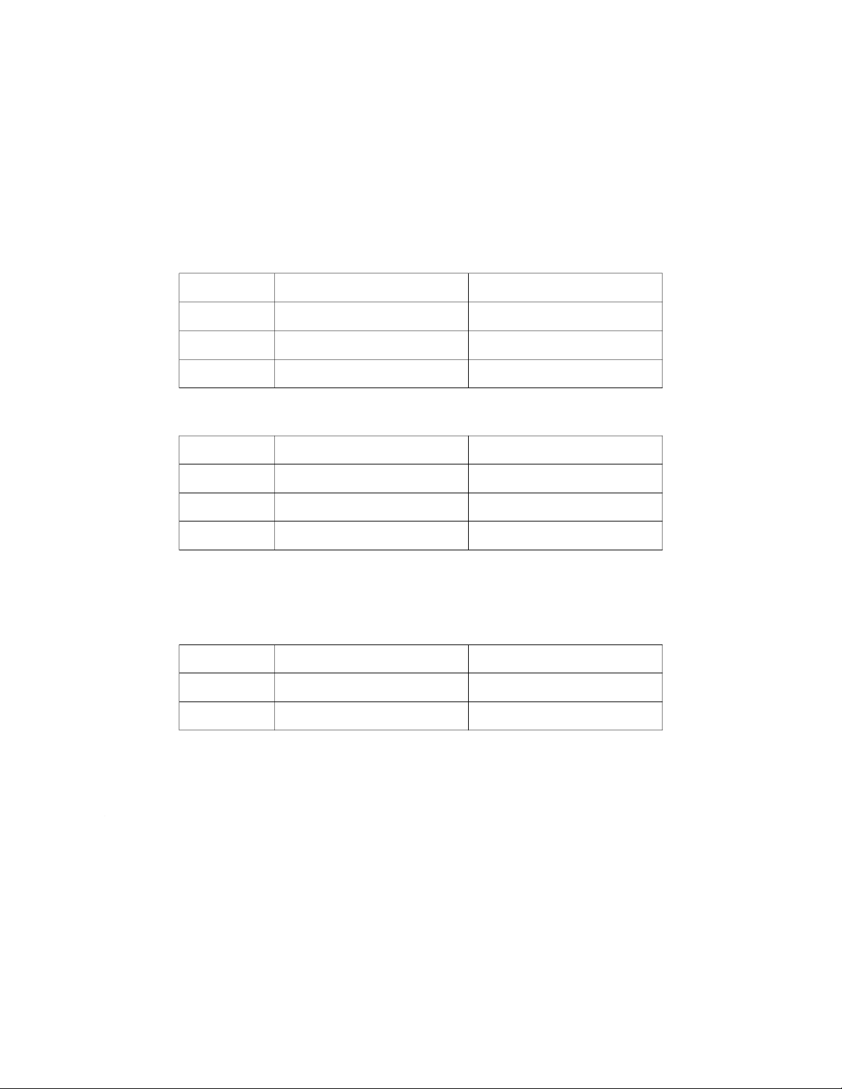
1) Measurement of unknown resistance: Trial f (Hz) R ( o Ω) 1 500 2187 2 1000 2169 3 1500 2180
2) Measurement of unknown capacitance: Trial f (Hz) R ( o Ω) 1 1000 230 2 2000 110 3 3000 75
3) Measurement of unknown inductance: Trial f (Hz) R ( o Ω) 1 50000 30 2 10000 54 2 3 150000 76
4) Measurement of resonant frequency of RLC circuit: Parellel RLC Circuit Series RLC Circuit Trial fs (Hz) fs (Hz) 1 6464 6503 2 6468 6489 3 6480 6515 II. Data Analysis:
1) Resistance Measurement: We have RX=R0 3 ∑ Ri i=1 Rx= 3=2178(Ω) 3 (Rxi−Rx )2 Δ Rx=S . D=
√∑i=13=7.4(Ω) Hence:
Rx=Rx± Δ Rx=2179±7.4(Ω)
2) Capacitance Measurement:
We have: CX=12πf R0
C1=6.91×10−7(F) ; C2=7,23×10−7(F) ; C3=7,07×10−7(F) 3 3 ∑ Cxi C i=1 X=
3=7.07×10−7(F) 3 (Cxi−Cx )2 Δ C X=S . D=
√∑i=13=0.13×10−7(F) Hence:
CX=(7,07±0.13)×10−7(F)
3) Inductance Measurement: We have: Lx=R0 2πf
L1=9.54×10−4(H) ; L2=8,59×10−4(H) ; L3=8.06×10−4(H) 3 ∑ Lxi i=1 L 3=8,73 x= ×10−4(H) 3 (Lxi−Lx )2 Δ L 3=0,51×10 x=S . D =
√∑i=1 −4(H) Hence:
LX= (8.73±0.51 )×10−4(H)
4) Determination of Resonant Frequency: a) Series RLC Circuit: 3 ∑ fxi i=1 fx= 3=6502(Hz)
√3∑(fxi −fx )2 Δ f i=1 X≈ S . D ≈ 3=10.6(Hz) 4 Hence:
fX−Series=6502±10.6(Hz)
b) Parallel RLC Circuit: 3 ∑ fxi i=1 fx= 3=6470(Hz)
√3∑(fxi−fx )2 Δ f i=1 x=S . D = 3=6.79(Hz) Hence:
fX−¿=6470±6.79(Hz)
c) Theoretical Result and Conclusion
We have: f=12π √LC fx=1
6.7×10−7×8.47×10−4=6406(Hz) 2π √
We can see that the theoretical result of resonant frequency is approximately equal to the directly
measured results. We can see that the RLC circuit (with properly small resistance) becomes a
good approximation to an ideal LC circuit. 5 6 Experimental Report 2
MEASUREMENT OF MAGNETIC FIELD INSIDE A SOLENOID WITH FINITE LENGTH I. Data Tables:
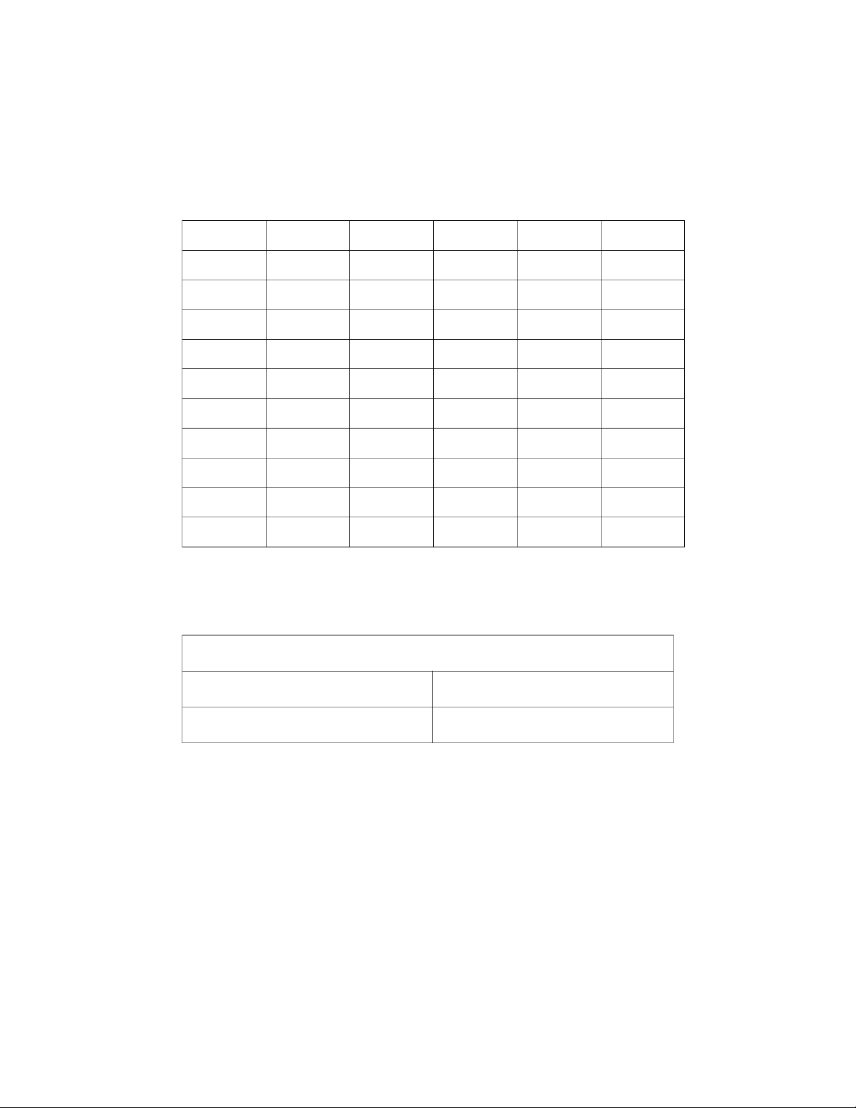
1. Investigation of the magnetic field at the position along the axis of solenoid: x (cm) B (mT) x (cm) B (mT) x (cm) B (mT) 1 1.29 11 1.74 21 1.74 2 1.5 12 1.74 22 1.73 3 1.6 13 1.74 23 1.72 4 1.66 14 1.74 24 1.71 5 1.69 15 1.74 25 1.70 6 1.71 16 1.74 26 1.67 7 1.72 17 1.74 27 1.63 8 1.72 18 1.74 28 1.55 9 1.73 19 1.74 29 1.38 10 1.73 20 1.74 30 0.98
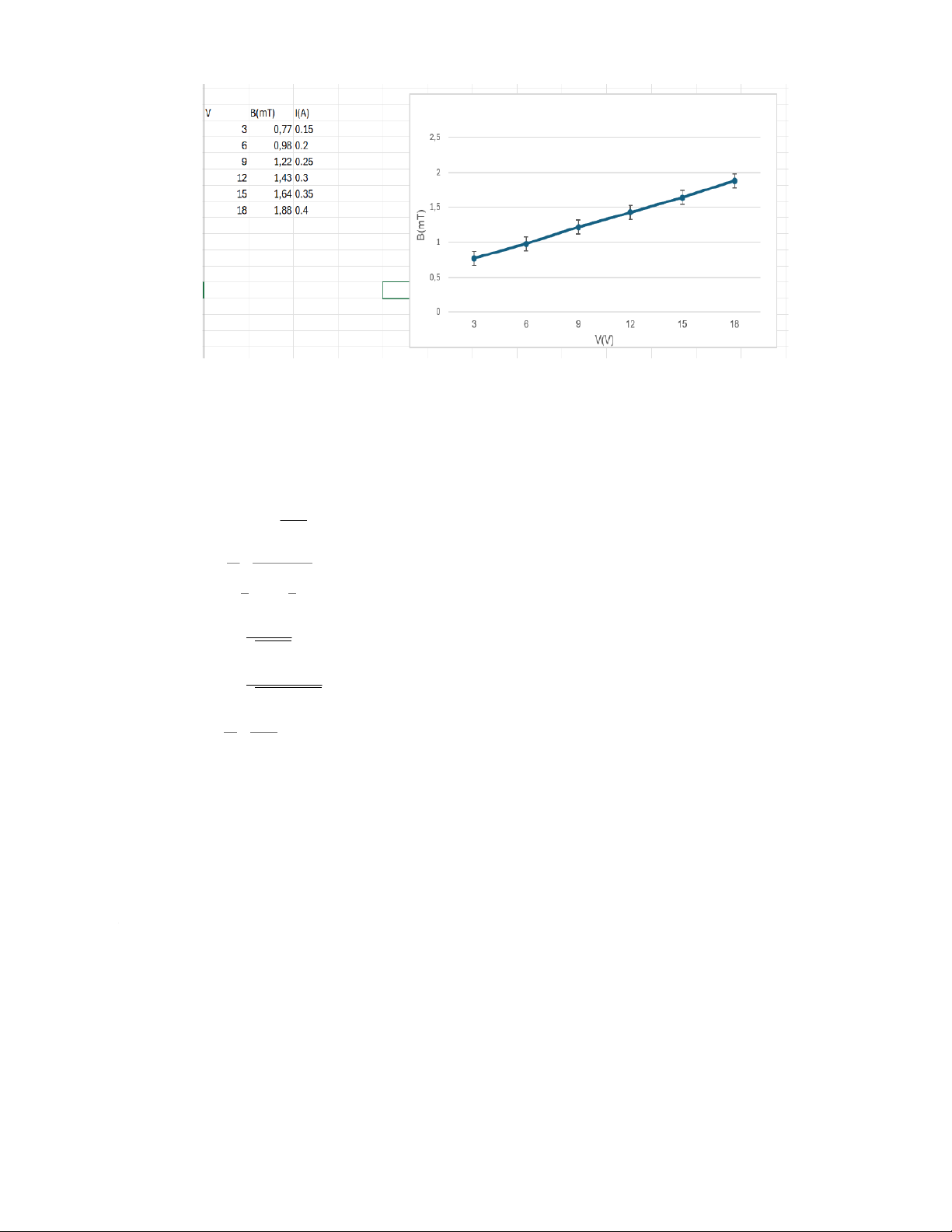
2) Measurement of the relationship between the magnetic field and the current through the solenoid: x = 15 (cm) I (A) B (mT) 0.15 0.77 7 0.2 0.98 0.25 1.22 0.3 1.43 0.35 1.64 0.4 1.88
3) Comparison of experimental and theoretical magnetic field: I = 0.4 (A) x (cm) B (mT) 0 0.85 10 1.8 20 1.79 30 0.93
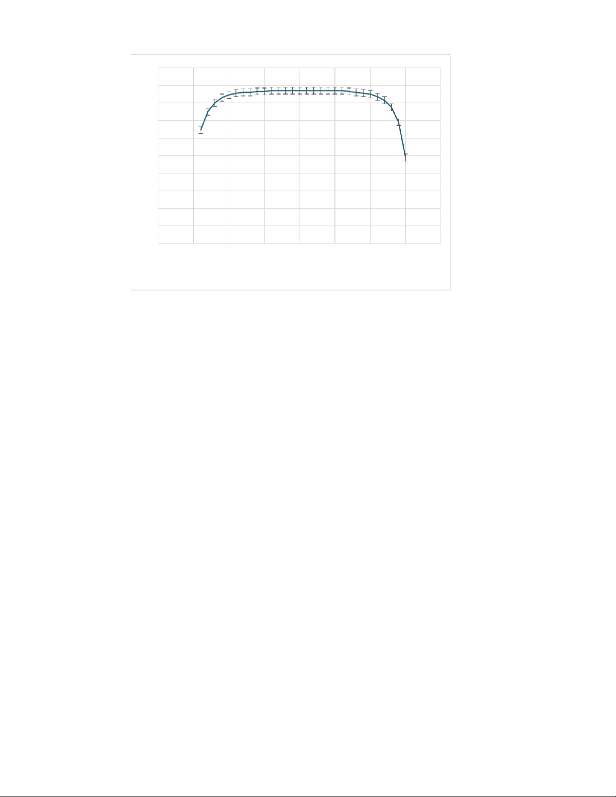
II. Relationship between the magnetic field and the position of the probe inside the solenoid: 8 2 1.8 1.6 1.4 1.2 1 B(mT) 0.8 0.6 0.4 0.2 0 -5 0 5 101520253035 x(cm)
The graph shows that the magnetic field inside a solenoid depends on the position of the probe
inside. The magnitude of the magnetic field increases from x=1 to x=8, and then stable until
x=21, then decreases at exactly the same pace as it increases. The graph is symmetric around the point x=15 (cm)
III. Relationship between the magnetic field and the applied voltage: 9
The graph shows that the magnitude of the magnetic field and the voltage has a linear
relationship. But in this case, the resistance is unchanged, so the current also has linear
relationship with the voltage. So, we can see that relationship between the magnetic field and the
applied current is also linear.
IV. Comparison of experimental and theoretical magnetic field:
We have: B=μ0μr
2. I . n0(cosγ1−cosγ2) ; μr=1 n0=NL=750 300×10−3=2500
I0=I √2=0.4 √2=0.566 (A) cosγ1=x√ R2+x2
cosγ2=−L−x √
R2+(L−x)2 R=D2=40.3 2=20.2(mm) a) x = 0 (cm):
cosγ1=0 ; cosγ2=−0.998 10 B=μ0μr =1.256×10−6
2I n0 (coscos γ1−coscosγ2 )
2×0.566×2500× (0+0.998 ) ¿0.87 (mT ) b) x = 15 (cm):
cosγ1=0.991 ; cosγ2=−0.991 B=μ =1.256×10 0μr −6
2I n0 (coscos γ1−coscosγ2 )
2×0.566×2500× (0.991+0.991) ¿1.76 (mT ) c) x = 30 (cm):
cosγ1=0.998 ; cosγ2=0 B=μ =1.256×10 0μr −6 2I n ) 0
(coscos γ1−coscosγ2 )
2×0.566×2500× (0.998−0 ¿0.87 (mT )
The result from the experiment is approximately close to the theoretical values from Data Table
3. The difference is due to the uncertainty of the instruments used. 11 Experimental Report 3
INDUCTOR AND FREE OSCILLATIONS IN RLC CIRCUIT
I. Resistance and Inductance of the Coil: - Graph: 12 - Data analysis: +Deduce variables: ▪Vs=1.016(V) ▪I0=0.10(A) ▪Slope S = 1417.48 +The resistance of the coil RL=VS =1.016 0.10=10.16(Ω) IO +Coil inductance
LW/O=RS=10.16
1417.48=7.17×10−3(H) 13 1) Free oscillation of RLC a. Frequency - Graph: - Data analysis: +Variables:
▪T=1.8×10−3(s)
▪LW/O=7.17×10−3(H)
▪C=10×10−6(T)
+The frequency based on the measurement fmeasured =1
T=11.8×10−3=555.56(Hz)
+The frequency based on theoretical calculations: fprediction=1 LC =1
7.17×10−3×10×10−6=594.37(Hz) 2π √ 2π √
+The difference between measurement and theoretical calculations: 14
Δ f =fmeasured −fprediction=555.56−594.37=−38.81(Hz) - The
experiment result is a bit different from the prediction result due to instrumental uncertainty. 2) Energy:
The total energy in RLC circuit:
U=Uc+UL=1 2C V 2+1 2L I 2 Comment:
- After stopping the electric power, the energy of the circuit does not decrease rapidly to
zero, it reduces to zero over a short period of time.
- The energy of oscillations of the coil and the capacitor are damped oscillations. Explain:
The energy of the circuit loses by the heat of the resistor at rate i2R
The graph of total energy is steepest at the time that the magnetic energy reaches a local
maximum because in these times, the current through the coil is highest, and the loss of energy is
mainly due to the resistance of the coil (ΔQ=i ). 2R 15 Experimental Report 4
VERIFICATION OF FARADAY’S LAW OF ELECTROMAGNETIC INDUCTION
I/Experiment Motivations
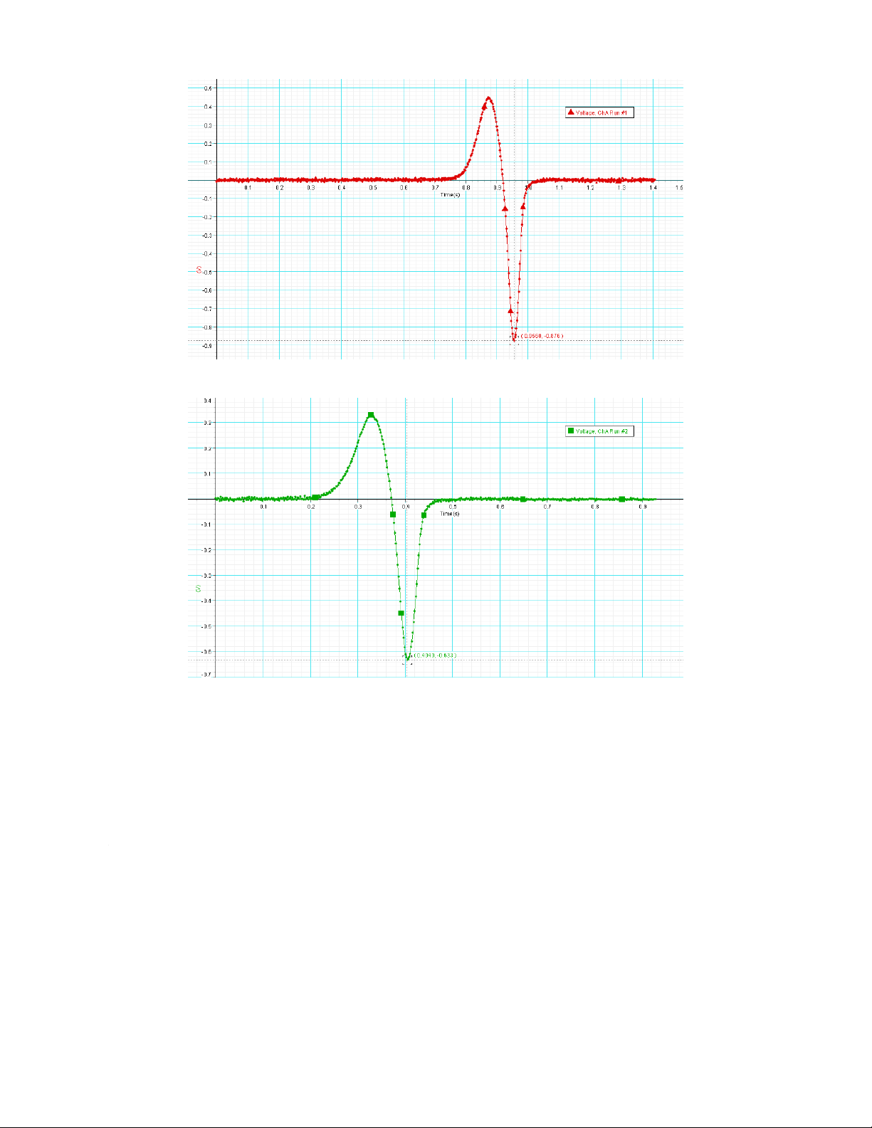
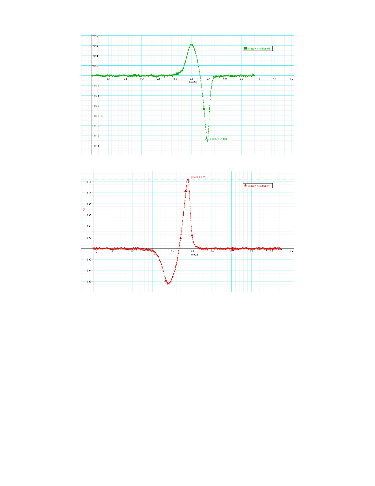
- Verify Faraday’s law of electromagnetic induction II/Experimental result 1)1200 turn coil R = 12 (Ω); L = 12 (mH) Pole Voltage Peak 1 Voltage Peak 2 North 0.434 -0.848 South -0.447 0.791 North-North 0.448 -0.867 South-South -0.482 0.775 North-South 0.328 -0.633 Graph North 16 South North-North 17 North-South South-South 18 2)150 turn coil Pole Voltage Peak 1 Voltage Peak 2 North 0.062 -0.831 South -0.064 0.125 North-North -0.052 -0.146 South-South -0.664 0.110 North-South 0.038 -0.103 Graph North 19 South North-South 20