
Preview text:
TE-2020-000227 1
A review of Quantum Neural Networks: Methods, Models, Dilemma Renxin Zhao1,2, Shi Wang1
1 College of Electrical and Information Engineering, Hunan University, Changsha, China
2 School of Mechatronics and Automotive Engineering, Huzhou Vocational and Technical College, Huzhou, China Abbreviation I. I CNN Classical Neural Network NTRODUCTION QNN Quantum Neural Network CELL
Quantum Cellular Neural Network NISQ
Noisy Intermediate-Scale Quantum
SINCE Feynman first proposes the concept of quantum
computers [1], technology giants and startups such as VQA Variational Quantum Algorithm
Google, IBM, and Microsoft have competed with each other, VQC Variational Quantum Circuit CV
Continuous-Variable architecture
eager to make it a reality. In 2019, IBM launches a quantum QP Quantum Perceptron
processor with 53 qubits, which can be programmed by SONN Self-Organizing Neural Network
external researchers. In the same year, Google announces that QSONN
Quantum Self-Organizing Neural Network QCPNN
Quantum Competitive Neural Networks
its 53-bit chip called Sycamore has successfully implemented CVNN Convolutional Neural Network
”Quantum Supremacy”. According to report, Sycamore can QCVNN
Quantum Convolutional Neural Network
complete the world’s fastest supercomputer IBM Summit in GAN Generative Adversarial Network
200 seconds to complete calculations that take 10,000 years to QGAN
Quantum Generative Adversarial Network GNN Graph Neural Network
complete, that is, quantum computers can complete tasks that QGNN Quantum Graph Neural Network
are almost impossible on traditional computers [2]. However, Qubit Quantum bit
this statement is quickly doubted by competitors including QCPNN
Quantum Competitive Neural Networks
IBM. IBM bluntly says: according to the strict definition of TNN Tensor Neural Network QTNN Quantum Tensor Neural Network
Quantum Supremacy, which means surpassing the computing RNN Recurrent Neural Network
power of all traditional computers, Google’s goal of achieving QRNN
Quantum Recurrent Neural Network
Quantum Supremacy has not been achieved. Therefore, IBM BM Boltzmann Machine QBM Quantum Boltzmann Machine
issues an article criticizing Google’s claim that traditional QWLNN
Quantum Weightless Neural Network
computers take 10,000 years to complete is wrong [3]. Since RUS Repeat-Until-Success
IBM found that it only takes 2.5 days after the deduction,
* By adding a lowercase letter s after the abbreviation to indicate their
it also commented that Google has intensified the excessive plural form
hype about the current state of quantum technology [3]. There
are still nearly ten years left until 2030, which is called
the first year of commercial use of quantum computing,
Abstract—The rapid development of quantum computer hard-
Quantum computers that can be produced at this stage are
ware has laid the hardware foundation for the realization of
arXiv:2109.01840v1 [cs.ET] 4 Sep 2021 QNN. Due to quantum properties, QNN shows higher storage all within the scope defined by NISQ. NISQ refers to the fact
capacity and computational efficiency compared to its classical
that there are fewer qubits available on quantum processors
counterparts. This article will review the development of QNN
recently, and quantum control is susceptible to noise, but it
in the past six years from three parts: implementation methods,
already has stable computing power and the ability to suppress
quantum circuit models, and difficulties faced. Among them, the
decoherence [4]. In short, quantum computers are the hardware
first part, the implementation method, mainly refers to some un-
derlying algorithms and theoretical frameworks for constructing
foundation for the development of QNN.
QNN models, such as VQA. The second part introduces several
QNN is first proposed by [5] and has been widely used in
quantum circuit models of QNN, including QBM, QCVNN and so
image processing [6]-[8], speech recognition [9][10], disease
on. The third part describes some of the main difficult problems
prediction [11][12] and other fields. For the definition of QNN,
currently encountered. In short, this field is still in the exploratory
stage, full of magic and practical significance.
there is no unified conclusion in the academic circles. QNN is
a promising computing paradigm that combines quantum com-
Index Terms—quantum neural networks, quantum computing,
puting and neuroscience [13]. Specifically, QNN establishes a
quantum machine learning, quantum circuit.
connection between the neural network model and quantum
theory through the analogy between the two-level qubits, the
Renxin Zhao is with Huzhou Vocational & Technical College, College
basic unit of quantum computing, and the active/resting states
of Mechanical and Electrical Engineering, No. 299 Xuefu Road, Huzhou,
in the complex signal transmission process in nerve cells [14].
313000, China. (e-mail:13061508@hdu.edu.cn)
At current stage, it can also be defined as a sub-category of
Shi Wang is with College of Electrical and Information Engineering, Hunan
University, Changsha, 410082, China. (e-mail: peoplews3@hotmail.com)
VQA, consisting of quantum circuits containing parameterized
Corresponding author: Shi Wang.
gate operations [15][16]. Obviously, the definition of QNN TE-2020-000227 2
can be completely different according to different construction
1995 to 2021, so this section mainly reviews the relatively
methods [17]-[22]. In order to further clarify the precise
mainstream methods in the past 6 years.
meaning of QNN, [23] puts forward the following three
preconditions: (1) The initial state of the system can encode
any binary string; (2) The calculation process can reflect the A. VQA
calculation principle of the neural network; (3) The evolution
VQC is a rotating quantum gate circuit with free parameters,
of the system is based on quantum effects and conforms to
which is used to approximate, optimize, and classify various
the basic theories of quantum mechanics. However, most of
numerical tasks. The algorithm based on VQC is called VQA,
the QNNs models currently proposed are discussed on the
which is a classical-quantum hybrid algorithm, because the
level of mathematical calculations, and there are problems
parameter optimization process usually takes place on classical
such as unclear physical feasibility, not following the evolution computers [15].
of quantum effects, and not having the characteristics of neural
The similarity between VQC and CNN is that they both
network computing. As a result, the real QNNs have not been
approximate the objective function by learning parameters, realized [23].
but VQC has quantum characteristics. That is, all quantum
From the perspective of historical development, QNN has
gate operations are reversible linear operations, and quantum
roughly gone through two main stages, namely the early stage
circuits use entanglement layers instead of activation functions
and the near-term quantum processor stage. In the early days,
to achieve multilayer structures. Therefore, VQC has been
QNN could not be implemented on quantum computers due
used to replace the existing CNN [16][33][41].
to hardware conditions. Most models were proposed based
A typical example is that, [16] defines QNN as a subset of
on the related physical processes of quantum computing, and
VQA and gives a general expression of QNN quantum circuit
did not describe specific quantum processor structures such as (see Fig. 1).
qubits and quantum circuits. Typical representatives are QNN
based on multiple world views [24], QNN based on interactive
quantum dots [25], QNN based on simple dissipative quantum
gates [26], QNN analogous to CNN [27], and so on. Compared
with earlier research results, the recently proposed QNN has
a broader meaning. The term QNN is more often used to
refer to a computational model with a networked structure
and trainable parameters that is realized by a quantum circuit
or quantum system [28]. In addition, the research of the QNN
model also emphasizes the physical feasibility of the model.
In the recent quantum processor stage, some emerging models
such as QBM [29]-[31], QCVNN [32]-[34], QGAN [35][36],
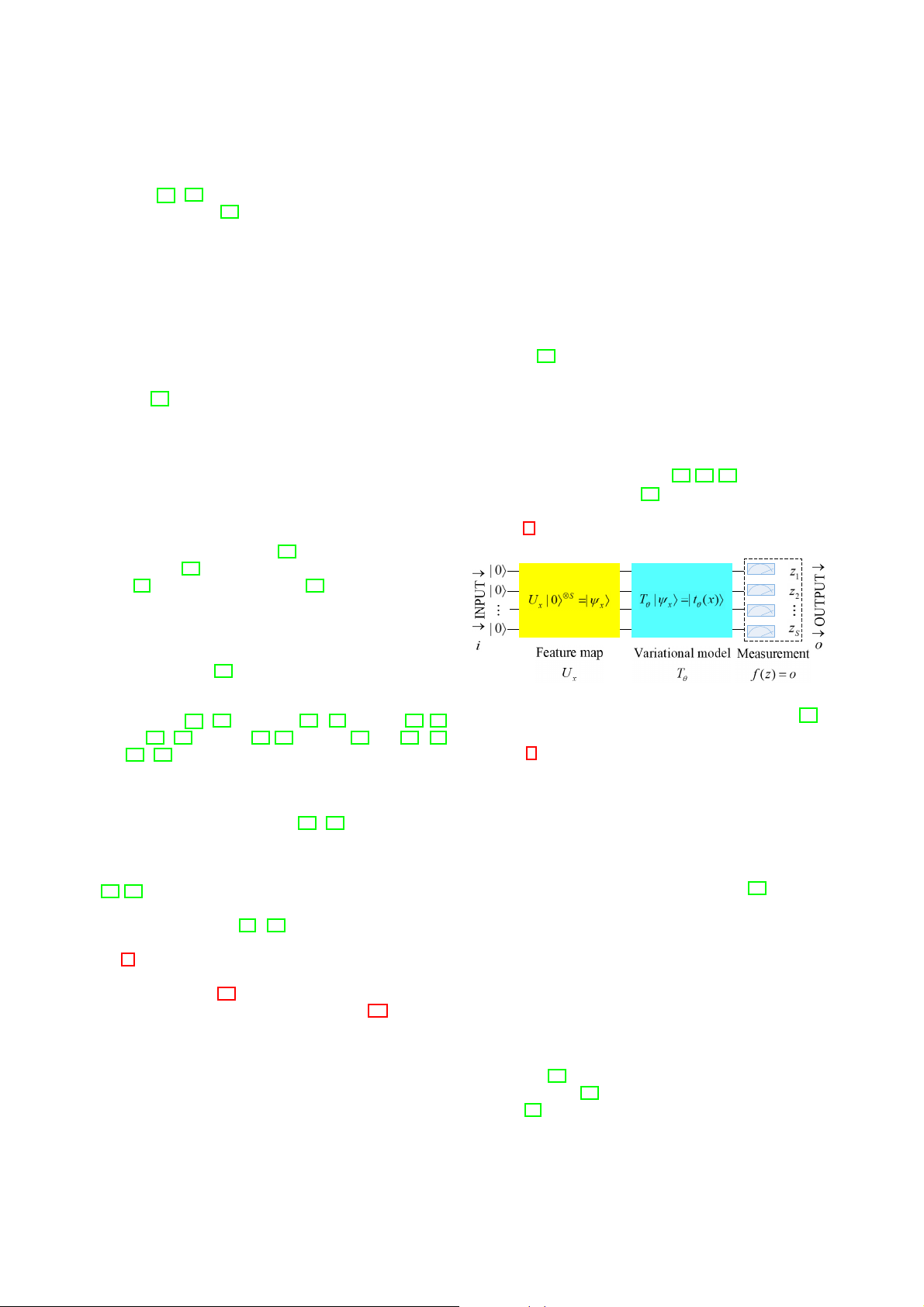
Fig. 1: QNN based on VQA framework modified from [16].
QGNN [37]-[39], QRNN [40][41], QTNN [42], QP[43]-[49],
etc. [50]-[60] will be introduced in subsequent sections.
In Fig. 1, in the first step, the quantum feature map method
QNN has surprising quantum advantages. But at this stage,
|ψx→ := Ux|0→⊗S encodes the input information i ∈ RSin which
the contradiction between dissipative dynamics in neural com-
is usually in the form of classical data, into the S-qubit
puting and unitary dynamics in quantum computing is still
Hilbert space. This step successfully realizes the transition
a topic worthy of in-depth study [61]-[67]. Furthermore, the
from classical state to quantum state. Subsequently, the VQA
current QNN can only be trained for some small samples
containing parameterized gate operations optimized for spe-
at low latitudes, and the prediction accuracy and generaliza-
cific tasks will play a role to evolve the obtained quantum
tion performance in large data sets is still an open problem
state into a new state, namely |tθ (x)→ := Tθ |ψx→, which is
[68][69]. In addition, it is also found that the barren plateau
similar to the classical machine learning process [16]. After the
phenomenon is easily formed in the parameter space of the
effect of VQA, the final output o := f (z) of QNN is extracted
QNN exponential level [70]-[73].
by quantum measurement. Before sending the information
Finally, the main work of this article is summarized. In Sec-
to the loss function, the measurement results z = (z0, . . . , zS)
tion II, the composition method of QNN will be introduced, so
are usually converted into corresponding labels or predictions
that readers have a preliminary understanding of the formation
through classic post-processing. The purpose of this is to filter
of QNN. In Section III, the QNN quantum circuit model for
the parameters θ ∈ Θ that can minimize the loss function for
the past six years will be introduced. In Section IV, some open VQA.
issues and related attempts will be introduced.
The VQA framework is one of the mainstream methods
for designing QNN. But it also inevitably inherited some of
VQA’s own shortcomings. For example, the QNN framework
II. SOME CONSTRUCTION METHODS OF QNN
proposed by [16], in some cases, is facing the crisis of barren
Many related reviews are very enthusiastic about the QNN
plateau. However, [16] does not give specific solutions. Addi-
model, but they do not systematically tell us how to build a
tionally, [16] does not investigate the measurement efficiency
QNN. This will be an interesting topic. In fact, it is extremely
of quantum circuits. Therefore, the QNN design under the
difficult to systematically summarize all the methods from
VQA framework is still worth exploring. TE-2020-000227 3 B. CV
The idea of CV comes from [28].CV is a method for encod-
ing quantum information with continuous degrees of freedom,
and its specific form is VQC with a hierarchical structure in-
cluding continuous parameterized gates. This structure has two
outstanding points, namely the affine transformation realized
by the Gaussian gate and the nonlinear activation function re-
alized by the non-Gaussian gate. Based on the special structure
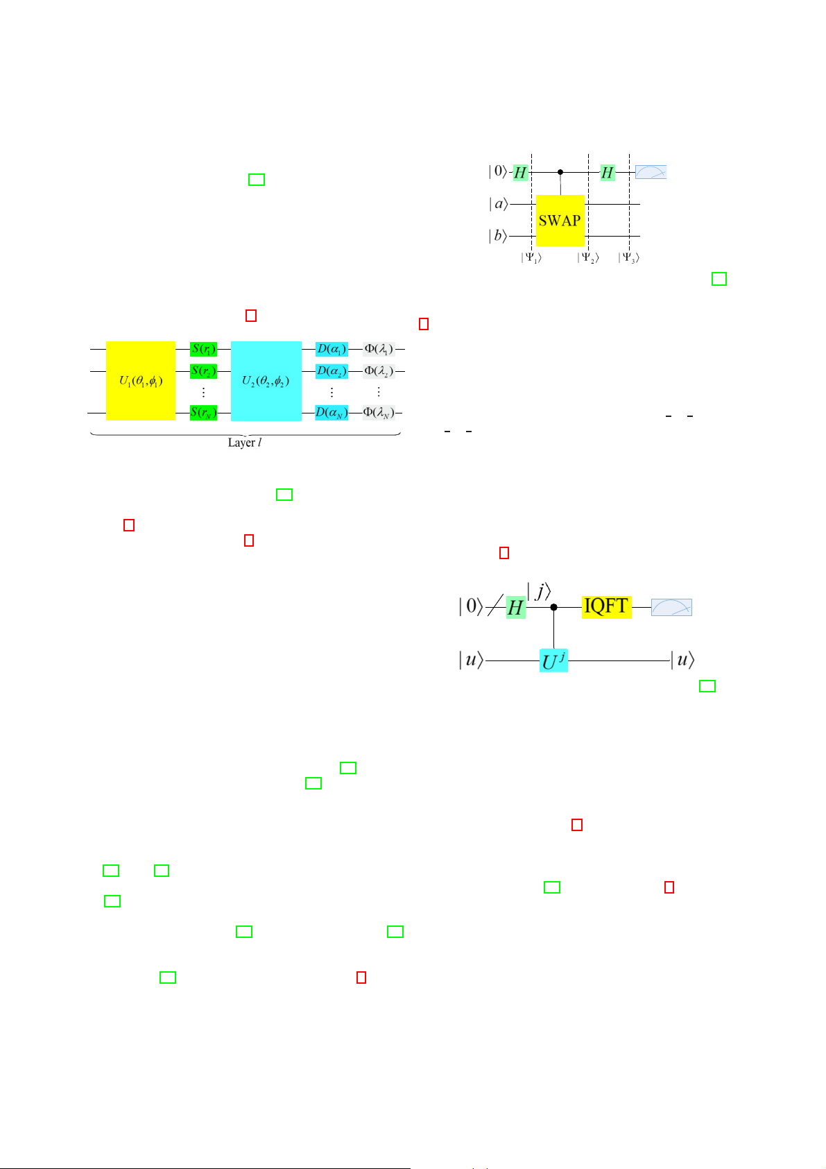
Fig. 3: Quantum circuit of a swap test modified from [18].
of the CV framework, highly non-linear transformations can be
encoded while retaining complete unity. The QNN framework
based on CV is shown in Fig. 2.
3 has two Hadamard gates and a controlled swap operator.
Assume that all states change to |Ψ1→ after going through the
first Hadamard gate. Subsequently, |Ψ1→ is further transformed
into |Ψ2→ under the action of the controlled swap operator.
Finally, apply the Hadamard gate again, and |Ψ3→ is obtained.
Performing projection measurement on ancilla qubits, we can
know that the probabilities of |0→ and |1→ are 1 + 1 |$a | b→|2 2 2
and 1 − 1 |$a | b→|2, respectively. Therefore, the square of the 2 2
inner product of qubits |a→ and |b→ can be expressed as |$a |
b→|2 = 1 − 2P(|1→), where P(|1→) represents the probability of
Fig. 2: A single layer QNN based on CV framework
when the ancilla qubit is in state |1→. modified from [28].
Phase Estimation Assuming that |u→ is an eigenvector of
the unitary operator U, the corresponding eigenvalue is e2iπϕ
Fig. 2 shows the l-th layer of the QNN model based on
and ϕ is undetermined. Our goal is to obtain the estimated
the CV framework. In Fig. 2 the universal N-port linear
value of ϕ through the phase estimation algorithm. As can be optical interferometers U
seen from Fig. 4, there are two quantum registers.
i = Ui(θi, φi) contain rotation gates
as well as beamsplitter. In this figure, S = ⊗N S(r i=1 i) repre-
sents squeeze operators, collective displacement is marked by D = ⊗N D(α i=1
i), and some non-Gaussian gates such as cubic
phase or Kerr gates are represented by the symbol Φ = Φ(λ ).
(θ , φ , r, α, λ ) are collective gate variables and free parameters
in the network, in which λ can have a fixed value. The
first interferometer U1, the local squeeze gate S, the second
interferometer U2 and the local displacement D are used for
affine transformation, and the last local non-Gaussian gate Φ
Fig. 4: Quantum phase estimation modified from [18].
is used for the final nonlinear transformation.
Being able to handle continuous variables is the bright
The first one contains t initial qubits with all states |0→,
spot of the CV-based QNN model, but one difficulty is how
and the second one starts in state |u→. The phase estimation
to realize the non-Gaussian gate, and to ensure that it has
algorithm is implemented in three steps. In the first step, the
sufficient certainty and tunability. In this regard, [28] does not
circuit first applies the Hadamard transformation to the first
give any further explanation. Moreover, [28] has only done
register, and then applies a controlled-U gates to the second
numerical experiments, and there is no practical application
register, where U is raised to successive powers of two. The case yet.
second step is to apply the inverse quantum Fourier transform
represented by IQFT in Fig. 4 to the first register. The third
step is to read the state of the first register by measuring on
C. Swap Test and Phase Estimation the basis of calculations.
[17] and [18] both suggest the method of swap test and
The QNN framework based on swap test and phase es-
phase estimation to build QNN. In the implementation scheme
timation proposed by [18] is shown in Fig. 5. This QNN
of [17], a single qubit controls entire input information of the
framework converts the numerical sample into a quantum
neuron during the swap test, which is not conducive to the
superposition state, and then obtains the inner product of
physical realization. Unlike [17], the quantum neuron in [18]
the sample and the weight through the swap test, and then
adopts the design of multi-phase estimation and multi-qubit
further maps the obtained inner product to the output of SWAP test.
the quantum neuron through phase estimation. According to
Swap Test [19] first proposes swap test (see Fig. 3).
reports, since the framework does not need to record or store
The meaning of this circuit is to know the square of the inner
any measurement results, it will not waste classical computing
product |$a | b→|2 of the qubits |a→ and |b→, by measuring the
resources. Although the model is more feasible to implement,
probability that the first qubit is in the state |0→ or |1→. Fig.
in the case of multiple inputs, the input space will increase TE-2020-000227 4
exponentially. Whether there will be a barren plateau is a
training. One feasible physical approach is to apply quantum question for further analysis. photonics.
Although the theory of [22] is universal, it ignores the non- D. RUS
linear problem when discussing the quantum generalization of QNN.
[20] uses the RUS quantum circuit [21] to achieve an
approximate threshold activation function on the phase of the
qubit, and fully maintain the unitary characteristics of quantum
III. ADVANCES OF QNN MODELS FOR NEAR-TERM evolution (see Fig. 6). QUANTUM PROCESSOR
A classic neuron can be seen as a function, which takes
n variables x1, . . . , xn and maps them to the output value A. QBM
o = f (w1x1 + . . . + wnxn + b), where {wi} and b are synaptic
[29] provides a new idea for the realization of QBM. Adopt-
weights and biases, respectively. f (·) is a non-linear activation
ing the input represented by the quantum state, employing
function, such as step function, sigmoid function, tanh func-
quantum gates for data training and parameter updating, by
tion, etc. We constrain the output value o to be -1 and 1, that
modeling the quantum circuits of visible layers and hidden is o ∈ [−1,1].
layers, the global optimal solution can be turned up by QRBM.
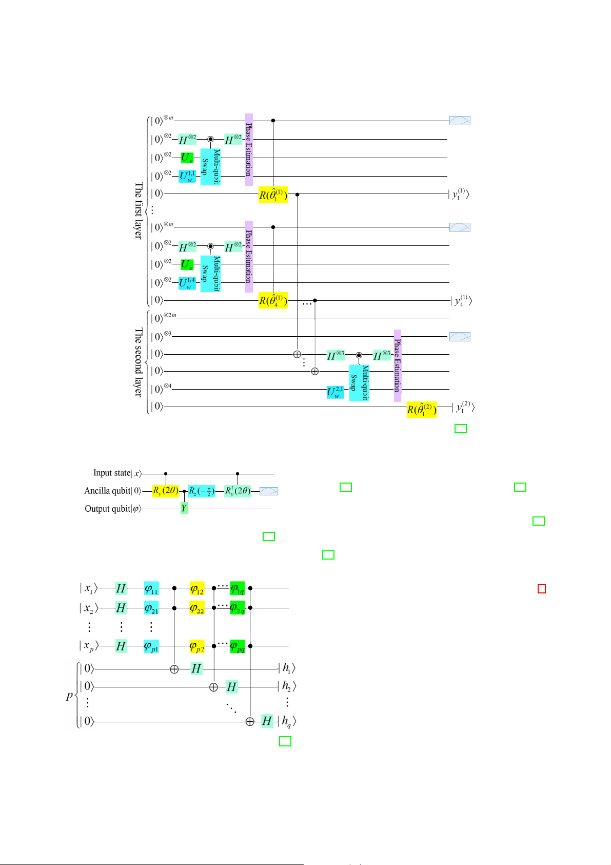
In order to map the above to the quantum framework, [20] (see Fig. 7).
introduces some necessary quantum states:
In Fig. 7, the visible layer variable is expressed as
1.Ry(b π + π )|0→ = cos(b π + π )|0→ + sin(b π + π )|1→, where 2 2 4 4 4 4 ( b ∈ [−1, 1] is a scalar;
|v1→,|v2→,··· ,|vp→), where
2.Ry(t) = e−itY/2 is a rotational quantum operation related 2π(vi − min1≤j≤p{vj}) to Pauli Y operator. |vi→ =cos( )|0→ max
Extreme cases, such as b = −1 and b = 1, will be mapped to
1≤ j≤p{v j} − min1≤ j≤p{v j} (1)
quantum states |0→ and |1→, respectively, and b ∈ (−1,1) will 2π(v + i − min1 sin( ≤ j≤p{v j}) )|1→
be regarded as a quantum neuron superimposed by |0→ and |1→.
max1≤j≤p{vj} − min1≤j≤p{vj}
Take |x→ = |x1 ...xn→ as the control state, and utilize Ry = (2wi) and i = 1, . . . , p. The hidden layer is denoted as
to the ancilla qubit conditional on the i-th qubit, and then apply (|h R
1→, |h2→, ··· , |hp→), where
y = (2b) to the ancilla qubit. This is equivalent to applying
Ry = (2θ ) to the ancilla qubit conditioned on the state xi of 2π(hk − min1≤I≤q{hl})
the input neuron. Rotation is performed by R ) y = (2 f (θ )) [20]. |hk→ = cos( |0→ max1
Fig. 6 depicts a circuit that carries out R
≤1≤q{hl} − min1≤I≤q{hl} y = (2 p(φ )), (2) 2π(h
where p(φ ) = arctan(tan2 φ ) is a nonlinear activation function. + k − min1 sin( ≤1≤q{hl}) )|1→
The measurement result of the ancilla qubit demonstrates
max1≤1≤q{hl} − min1≤l≤q{hl}
the influence of the RUS circuit on the output qubit. The
and k = 1, . . . , q. The quantum register has p qubits. The
measurement returns to |0→, denoting that the rotation of
Hadamard gate in Fig. 7 is used for preprocessing [29]. The
2pok(φ ) is successfully achieved to the output qubit. On the
coefficients of the visible layer variables are changed with the
contrary, if it is |1→, Ry(π/2) is rotated on the output qubit. At
phases of a series of quantum rotation gates. The quantum
this time, Ry(−π/2) needs to be used to offset this rotation.
state of each variable is switched through the CNOT gate, and
Then the circuit keeps repeating until |0→ is detected on the
the entire variable in the visible layer is summed into one
ancilla qubit, which is why it is called RUS
qubit [29]. After passing through the Hadamard gate again,
The highlight of [20] is to use quantum circuits to approxi-
the quantum state of a qubit in the hidden layer is obtained to
mate nonlinear functions, that is, to solve nonlinear problems represent the output.
by linear means. This unifies nonlinear neural computing and
In recent years, QBM models based on variable quantum
linear quantum computing, and meets the basic requirements
algorithm have also been proposed. [30] proposes a variational
of [23]. It is also worth mentioning that RUS is a flexible
virtual-time simulation based on NISQ equipment to realize
way. Quantum neurons constructed with RUS also have the
BM learning. It is different from the previous method of
potential to construct various machine learning paradigms,
preparing thermal equilibrium, but uses a pure state whose
involving supervised learning, reinforcement learning and so
distribution simulates the thermal equilibrium distribution. It on.
has been proved that NISQ equipment has the potential of
effective use in BM learning. [31] prepares the Gibbs state E. Quantum generalization
and evaluates the analytical gradient of the loss function based
[22] puts forward a quantum generalization method for
on the variable quantum virtual time evolution technology.
CNN, that is, the reformation of the perceptron can be ex-
Numerical simulations and experiments are carried out on IBM
plained by each reversible and unitary transformation in QNN.
Q to prove the approximation of the variational Gibbs state.
Through the use of numerical simulations, it has been proven
Compared with [30] and [31], [29] realized a pioneering effort
that gradient descent can be used to train for a given objective
to realize QBM with quantum gates, explored the appropriate
function. Minimizing the difference between the expected
number of hidden layers, and tested the pattern recognition
output and the output of the quantum circuit is the purpose of
performance of gearboxes with different hidden layers. TE-2020-000227 5
Fig. 5: QNN based on swap test and phase estimation framework modified from [18]. B. QCVNN
QCVNN has received extensive attention in the past three
years. [32] first mentiones the term QCVNN. In [32], the
input information is represented by qubits, which are trained
under the CVNN framework, and the probability of a certain
Fig. 6: Repeat-until-success (RUS) circuit for realizing
characteristic state is obtained by measurement. But what [32]
rotation with an angle p(φ ) = arctan(tan2 φ ). [20].
puts forward is only a theoretical model, which does not have
the feasibility of quantum circuits.
[33] designs a quantum circuit model of QCVNN, which
implements convolution and pooling transformation similar
to CVNN for processing one-dimensional quantum data. The
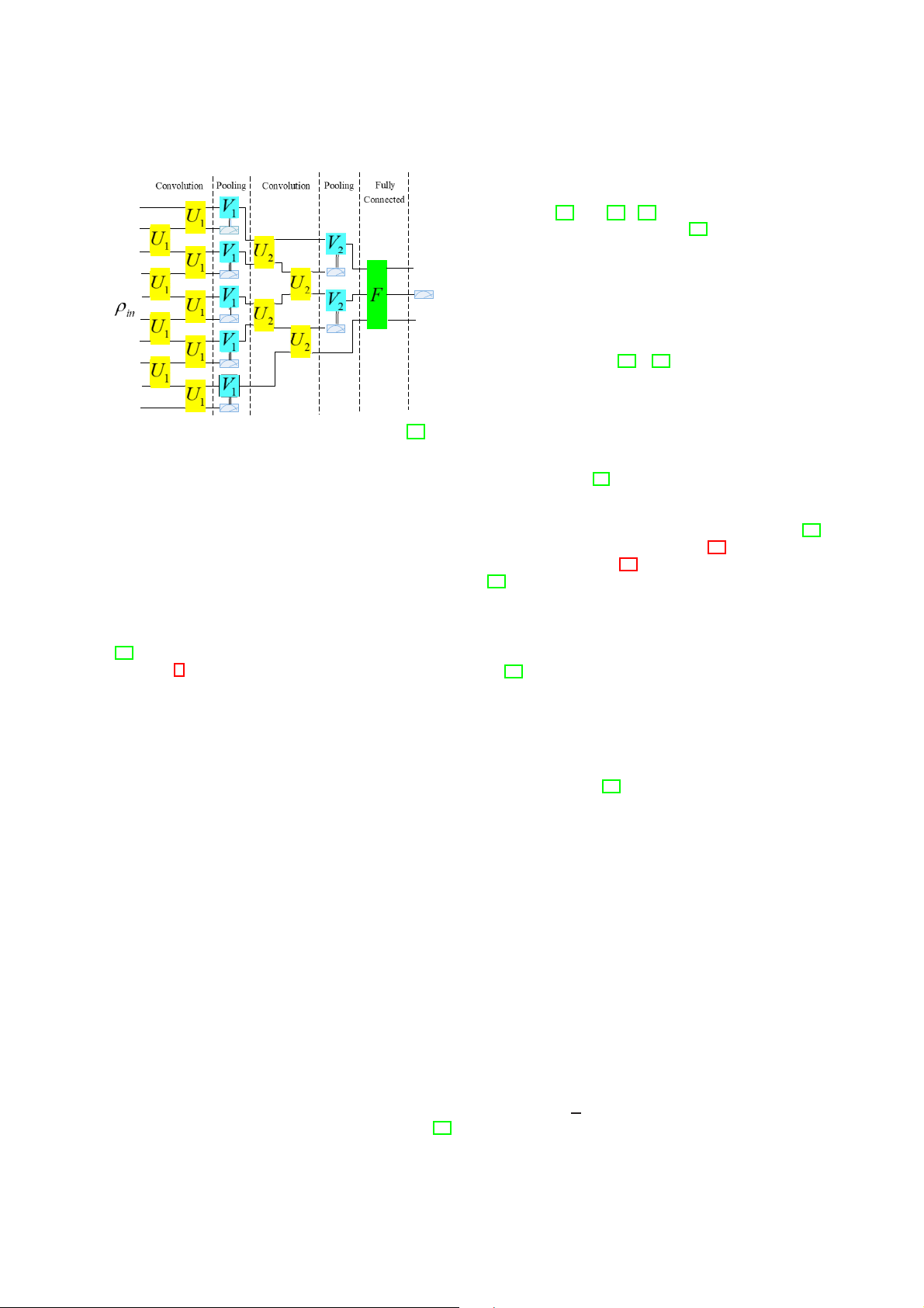
quantum circuit structure of QCVNN is shown in Fig. 8,
including several repeated convolutional layers and pooling
layers, as well as a fully connected layer.
The convolutional layer imposes a finite depth of quasi-local
unitary transformation, and each unitary transformation param-
eter in the same convolutional layer is the same. The pooling
layer measures some qubits and applies classical controlled
unitary transformation on adjacent qubits. The parameters of
the unitary transformation depend on the measurement results
of adjacent qubits. After multi-layer convolution and pooling
transformation, when there are few remaining qubits, a unitary
transformation is applied as a fully connected layer, and the
specified qubits are measured to obtain the judgment result
of the network. Each convolutional layer and pooling layer
Fig. 7: The quantum circuit of QRBM modified from [29].
of the network share the unitary transformation of the same
parameter, so for n-bit input qubits, it only has parameters of TE-2020-000227 6
the optional step size and nucleus still need to be further probed.
Comparing [33] and [34], [33] only gives a QCVNN model
for low-dimensional input. Although [33] also mentiones that
the proposed model is extensible, it does not elaborate on
the expansion steps. Relatively speaking, the input dimension
discussed by deep QCVNN is higher. C. QGAN
The concept of quantum generative adversarial learning
can be traced back to [35]. [35] discourses the operating
efficiency of quantum generative adversarial learning in a
variety of situations, such as the training data is classical data
or quantum data, and whether the discriminator and generator
Fig. 8: The structure of QCVNN modified from [33].
use quantum processors to run. Reportedly, when the training
data is quantum data, the quantum confrontation network may
show an exponential advantage over the classical confrontation
the order of O(log(n)), which can be efficiently trained and
network. However, [35] does not give a specific quantum
deployed on quantum computers in near term. In addition, the
circuit scheme, nor does it conduct a rigorous mathematical
pooling layer can reduce the dimensionality of the data and derivation.
introduce a certain non-linearity through partial measurement.
A quantum circuit version of GAN is proposed by [36].
It is worth noting that as the convolutional layer increases,
The schematic diagram is shown in Fig. 10 and the structure
the number of qubits spanned by the convolution operation diagram is shown in Fig. 11.
will also increase. Therefore, the deployment of the QCVNN
[36] assumes that there is a data source (S) and a label
model on a quantum computer requires the ability to imple-
|φ→ is given, and the density matrix ρSφ is output to a register
ment two-qubit gates and projection measurements at various
comprising n subsystems, namely distances. R(|φ→) = ρS
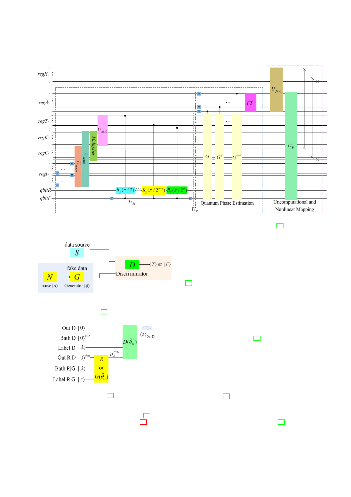
[34] introduces a deep QCVNN model for image recogni- φ (3)
tion (see Fig. 9). The general working principle of the model is
In [36], the essence of the Generator (G) is VQC, and its
that the input image will be encoded into quantum states with
gate is parameterized by the vector !θG. Regarding the label |φ→
basis encoding, and then these quantum states undergo a series
and the additional state |a→ as inputs, G generates a quantum
of parameter-related unitary transformations to realize the state
quantum evolution process. Unlike CVNN, this model omits G(!θG, |φ, a→) = ρG φ (! θG, a) (4)
the pooling layer, only retains the quantum convolution layer
and quantum classification layer, and increases the convolution In (4), ρG
φ is output on a register containing n subsystems,
step size to 2m to finish sub-sampling. This is advantageous
similar to the real data [36]. The additional input state |a→ has a
to remove the intermediate measurement, so as to achieve the
dual role. On the one hand, it can be seen as an unstructured
purpose of quickly reducing the dimension of the generated
noise source that supplies entropy in the distribution of the
feature map. Finally, the corresponding classification label is
generated data. On the other hand, it can be regarded as a
acquired through quantum measurement. For some details, control for G.
for example, in the quantum convolution layer, the quantum
The training signal of G is given by the Discriminator (D),
preparation of the input image and the related convolution
which consists of an independent quantum circuit parameter-
kernels is performed by the QRAM algorithm. For another
ized by the vector !θD. The function of D is to judge whether
example, the quantum inner product operation of the kernel
the given input state comes from S or G. During this period, G
working area requires the support of a quantum multiplier and
will deceive D continuously, and try its best to make D believe
a controlled Hadamard gate rotation operation. Furthermore,
that its output is True (T, ”Fake” denoted as F). Assuming
the conversion between amplitude coding and base coding
the input is from S, the output register of D will output |T →,
and nonlinear mapping are determined by the quantum phase
otherwise it will output |F→. In the internal work area, D can
estimation algorithm. Finally, by separating the desired state
also perform operations. So as to cpompel G to comply with
and the intermediate state, non-computational operations are
the provided label, D is also given a copy of the unchanged
employed to obtain the input state of the next layer. label.
The proposal of the deep QCVNN model proves the feasi-
Adversarial tasks can describe the optimization goals of
bility and efficiency in multi-type image recognition. However, QGAN
this model can only limit the size of the input image to the 1 φ
range of 2n × 2n. Once it is not in this range, the image needs min max ∑ Pr((D(!θ φ
D, |φ →, R(|φ →)) = |T →)
to be scaled additionally. For the image scaling problem, [34] !θ ¯ θ (5) G D φ =1
does not give a good quantum version solution. Furthermore,
∩ (D(!θD,|φ→,G(!θG,|φ,a→)) = |F→)) TE-2020-000227 7
Fig. 9: The quantum circuit for the convolutional layer in deep QCVNN model modified from [34].
the parametrized G G(!θG). The initial resource state |0,0,λ →
defined in the Out D, Bath D and Label D registers and the information ρS/G φ
from S are available for D D(!θD) to use.
D announces whether the result is |T → or |F→ in the Out D
register. The expected value $Z→Out D is proportional to the
probability that D will output |T →.
[36] proved the feasibility of QGAN’s explicit quantum
circuit through a simple numerical experiment. QGAN has
more extensive characterization capabilities than the classic
version, for example, it can learn to generate encrypted data.
Fig. 10: The schematic diagram of QGAN modified from [36]. D. QGNN
A deep learning architecture that can directly learn end-
to-end, Quantum Space Graph Convolutional Neural Network
(QSGCNN), was proposed by [37] to classify graphs of
any size. The main idea is to transform each graph into a
fixed-size vertex grid structure through the transfer alignment
between graphs, and use the proposed quantum space graph
convolution operation to propagate the vertex features of the
grid. According to reports, the QSGCNN model not only
retains the original map features, but also bridges the gap
between the spatial map convolutional layer and the traditional
Fig. 11: The general structure diagram of QGAN modified
convolutional neural network layer, and can better distinguish from [36]. different structures [37].
Quantum Walking Neural Network (QWNN), a graph neural
network structure based on quantum random walk, constructs
After clarifying G, D and optimization goals, [36] gives the
diffusion operators by learning quantum walks on the graph,
general structure of QGAN, as shown in Fig. 11. The initial
and then applies them to graph structure data [38]. QWNN can
states are respectively defined on the registers labeled Label
adapt to the space of the entire graph or the time of walking.
R|G, Out R|G and Bath R|G, which can be applied by S or
The final diffusion matrix can be cached after learning has TE-2020-000227 8
converged, so that it can be quickly advanced in the network. E. QRNN
However, due to the constant shift operation and coin insertion
[40] constructs a parameterized quantum circuit similar to
in the learning process, this model is significantly slower than
the RNN structure. Some qubits in the circuit are used to
other models. Space complexity is called a problem worthy of
memorize past data, while other qubits are measured and continued analysis.
initialized at each time step to obtain predictions and encode
The above models belong to the theoretical framework. The
a new input data. The specific structure is shown in Fig. 13.
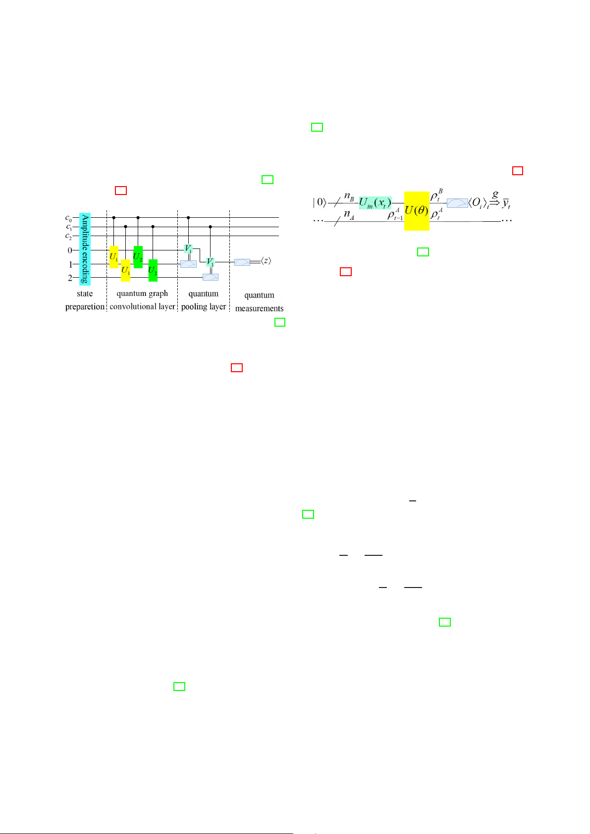
quantum circuit model of QGNN was studied by [39], as shown in Fig. 12.
Fig. 13: Structure of QRNN for a single time step modified from [40].
In Fig. 13, there are two groups of qubits, denoted by
nA and nB respectively. The qubits of group A have never
been measured, and they are used to retain past information.
The qubits of group B are measured every time step t, and
initialized at the same time to output prediction and input to the
Fig. 12: A QGCN quantum circuit model modified from [39].
system. The time step here is composed of three parts, namely
the encoding part, the evolution part and the measurement
Quantum state preparation, quantum graph convolutional
part. In the encoding part, Uin(xt ) is used for the initial state
layer, quantum pooling layer and quantum measurements
|0→ (abbreviate |0→⊗nB as |0→), and the training data xt is
constitute the quantum circuit model of Fig. 12. In the state
encoded into the quantum state of the B group of qubits.
preparation stage, the image data is effectively encoded into a
The information about x0, . . . , xt−1 has been saved in group A
quantum state by the amplitude encoding method. The normal- as the density matrix ρA = (θ , x t−1
0, . . . , xt−1) generated in the
ized classical vector x ∈ C2n,∑j |x j|2 = 1 can be represented
previous step. In the evolution part, the parameterized unitary
by the quantum state |ψ→ as follows:
operator U (θ ) acts on the entire qubit, which can transfer
information from group B to group A. Here, use the evolved 2n ρA x = (x t and ρB t
to represent the simplified density matrices of A
1, . . . , x2n )T → |ψx→ = ∑ x j| j→ (6)
and B, respectively. In the measurement part, first measure the j=1
expected value of a group of observations {Oi} in group B to
In the same way, a classic matrix B ∈ C2n×2m with obtain a $O i j that satisfies ∑ i→t = Tr[ρ B
i j |ai j |2 = 1 can be encoded as |ψ → = t Oi] (7) ∑2m i=1 ∑2n
j=1 ai j |i→| j→ by expanding the Hilbert space accordingly.
Then, the expected value is transformed into a certain
In the quantum graph convolutional layer, the constructed
function g, and the prediction yt = g({$Oi→t}) of yt is obtained.
dual-qubit unitary operation U realizes local connection. The
[40] points out that the transformation g can be chosen
number of layers of the quantum graph convolutional layer in-
arbitrarily, for example, g can be a linear combination of
dicates the order of node aggregation, so the unitary operations
{$Oi→t}. Finally, the qubits in group B are initialized to |0→.
of the same layer have the same parameters, which reflects the
After repeating these three parts many times, y0, . . . , yT−1’s
characteristics of parameter sharing. In the quantum pooling
prediction y0, . . . , yT−1 can be obtained. After the prediction is
layer, quantum measurement is added to reduce the feature
obtained, the cost function L is calculated, which represents
dimension, achieving the same effect as the classical pooling
the difference between the training data {y0,... ,yT−1} and
layer. Note, however, that not all qubits are measured, but
the predicted data {y0,...,yT−1} obtained by QRNN. The
a part of it is measured. Based on the measurement results,
parameter θ is optimized by a standard optimizer running on
it is determined whether to perform unitary transformation
a classic computer to minimize L.
on adjacent qubits. Finally, after multi-layer convolution and
The QRNN model proposed by [40] is a parameterized
pooling transformation, the specified qubit can be measured
quantum circuit with a recursive structure. The performance
by quantum, and the expected value can be obtained. The
of the circuit is determined by three parts: (1) different data
results show that the structure can effectively capture node
encoding units (2) the structure of the parameterized quantum
connectivity and learn the hidden layer representation of node
circuit (3) the optimizer used to train the circuit. For the features.
first point, a simple door is used as a demonstration in the
The model proposed by [39] can effectively deal with
article. For the second point, we can still explore further. For
the problem of graph-level classification. The four major
the third factor, we can learn from the method of VQA. But
structures can effectively capture the connectivity of nodes,
an unresolved question is whether QRNN is better than the
but currently only the node information is used, and the
classic one. This problem requires the establishment of some
characteristics of edges are not studied.
indicators for further analysis and experimentation. TE-2020-000227 9 F. QTNN
it seems to have application potential in the noise recovery
[42] is the first to explore quantum tensor neural networks
ability of machine learning algorithms. In addition, tensor
for recent quantum processors (see Fig. 14).
network is a very promising framework because it has achieved
a careful balance between expressive power and computational
efficiency, and has rich theoretical understanding and powerful optimization algorithms. G. QP
QP is one of the relatively mature models. The smallest
organ of QP is a quantum neuron [20]. [43] establishes a
model of neuron and concludes: a single quantum neuron
can perform an XOR function that cannot be achieved by
a classical neuron, and has the same computing power as a
double-layer perceptron. Quantum neurons also have variants
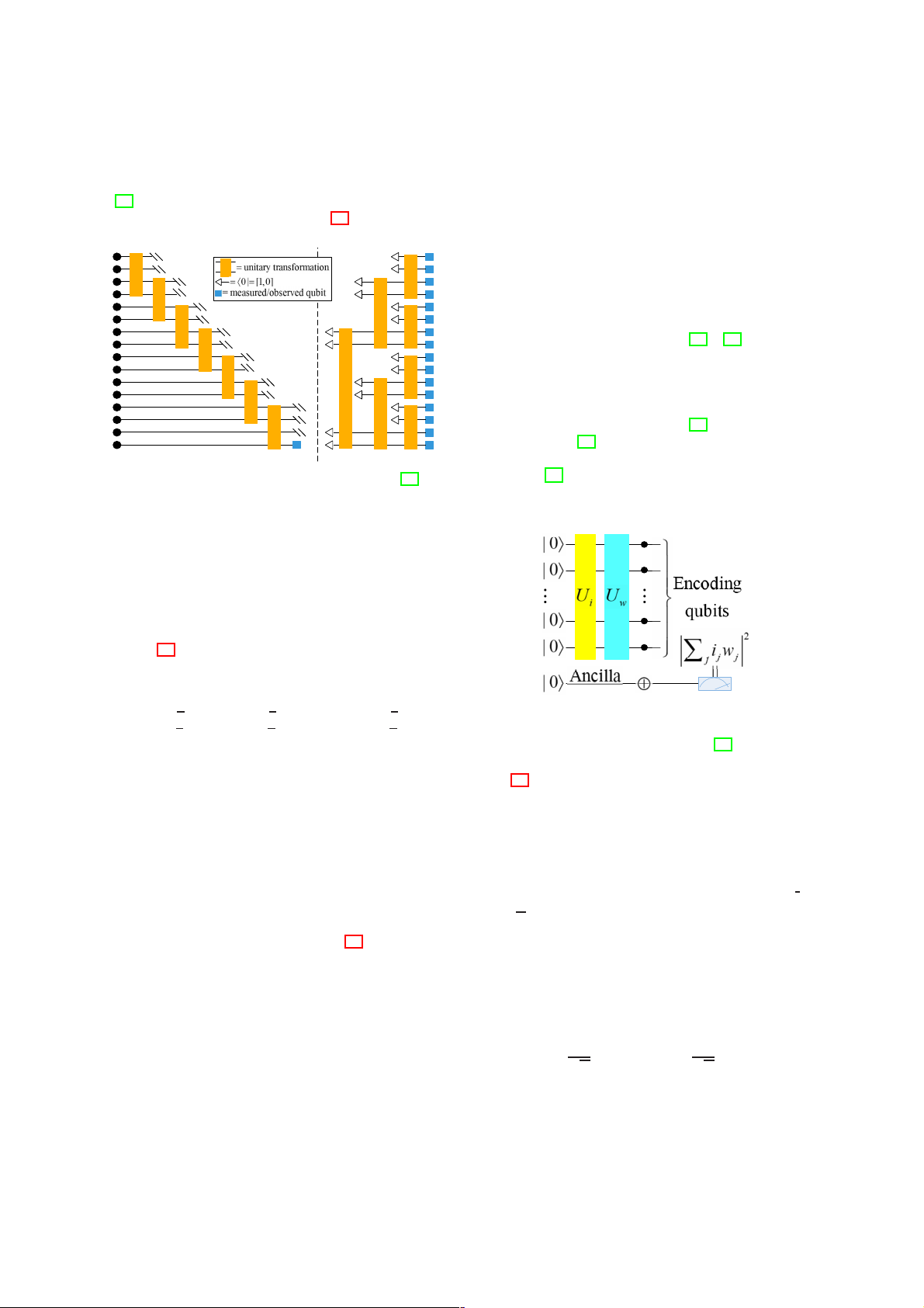
such as feedback quantum neurons [44] and artificial spike quantum neurons [45]. (a) (b)
In view of the core position of neurons in the multilayer
Fig. 14: Quantum tensor networks modified from [42]. (a)
perceptron, [46] proposes an artificial neuron that can be
The discriminative network; (b) the generative network.
carried out an real quantum processor. The circuit it provides is as follows.
The author proposes a QNN with a tensor network structure,
which can be used for discrimination tasks and generation
tasks. The neural network model has a fixed tree structure
quantum circuit, in which the parameters of the unitary trans-
formation are not fixed initially, and the training algorithm
is a quantum-classical hybrid algorithm, that is, searching for
suitable parameters with the aid of a classical algorithm.
In Fig. 14 (a), the discriminant model encodes the input
data x = (x1, ··· xn),0 ≤ xi ≤ 1 as a product state of n qubits, as the input quantum state cos( π x cos( π x cos( π x
Fig. 15: Scheme of the quantum algorithm for the |x→ = ( 2 1) ) ⊗ ( 2 2) ) ⊗ ··· ⊗ ( 2 n) ) (8) sin( π x sin( π x sin( π x
implementation of the artificial neuron model on a quantum 2 1) 2 2) 2 n) processor, modified from [46]
The quantum circuit of the discriminant model is similar to
a multilayer tree structure. After applying the unitary trans-
Fig. 15 outlines the principle. The system starts from the
formation, half of the qubits are ignored, and the remaining
state |00 ...→, and after passing through the unitary matrix |ψ
qubits continue to participate in the operation of the next i→,
|00...→ is transformed into the input quantum state |ψ
layer of nodes. Finally, one or more qubits are used as output i→. |ψi→ undergoes transformation U
qubits, and the most probable measurement result is used as
w, transfers the result to an ancilla
qubit, and finally performs quantum measurement on it to
the judgment result of the input data by the neural network. In
assess the activation state of the perceptron.
the training process, the classical algorithm is used to compare
More specifically, the input vector and weight are restricted
the discrimination result with the real label, and the circuit to the binary value i
parameters are updated according to the error.
j , w j ∈ {−1, 1}. Given any input i and
weight w vector, use m coefficients required to define the
The generative model adopts a structure almost opposite to general wave function |ψ
the discriminant model, as shown in Fig. 14 (b). The newly
i→ of N qubits to encode the m- dimensional input vector.
added qubit is combined with the original qubit to participate
in the calculation of the lower unitary transformation node. ¯i = (i0,... ,im−1)T (9)
After generating the required number of qubits, the data ¯ w = (w0, . . . , wm−1ight)T with i j, w j ∈ {−1,1}
information generated by the QNN model is obtained through
measurement. When training the network, the quantum cir-
Next, two quantum states are defined
cuit parameters are also adjusted through classical algorithms 1 m−1 1 m−1
according to the generated results and label errors. |ψi→ = √
∑ ij| j→,|ψw→ = √ ∑ wj| j→ (10) m m
The tensor network provides an increasingly complex natu- j=0 j=0
ral hierarchical structure of quantum states, which can reduce
where | j→ ∈ {|00 ...00→,|00 ...01→,...,|11 ...11→}. As de-
the number of qubits required to process high-dimensional data
scribed in (10), the factor ±1 can be used to encode the m-
with the support of dedicated algorithms. In addition, it can
dimensional classical vector as a uniform weighted superpo-
alleviate the problems related to random initial parameters, and
sition of the complete calculation basis | j→. TE-2020-000227 10
First, encode the input value in i to prepare the |ψi→ state.
and O(nk) quantum gates, where n is the number of input
Assuming that the initial state of the qubit is |00 ···00→ ≡
parameters and k is the number of weights applied to these
|0→⊗N, a unitary transformation Ui is performed such that
parameters. The corresponding quantum circuit is drawn as follows. Ui|0→⊗N = |ψi→ (11)
In principle, any m × m unitary matrix with i in the first
column can be used for this purpose. In a more general case,
starting from a blank register to prepare the input state may be
replaced by the quantum memory stored before |ψi→ is directly
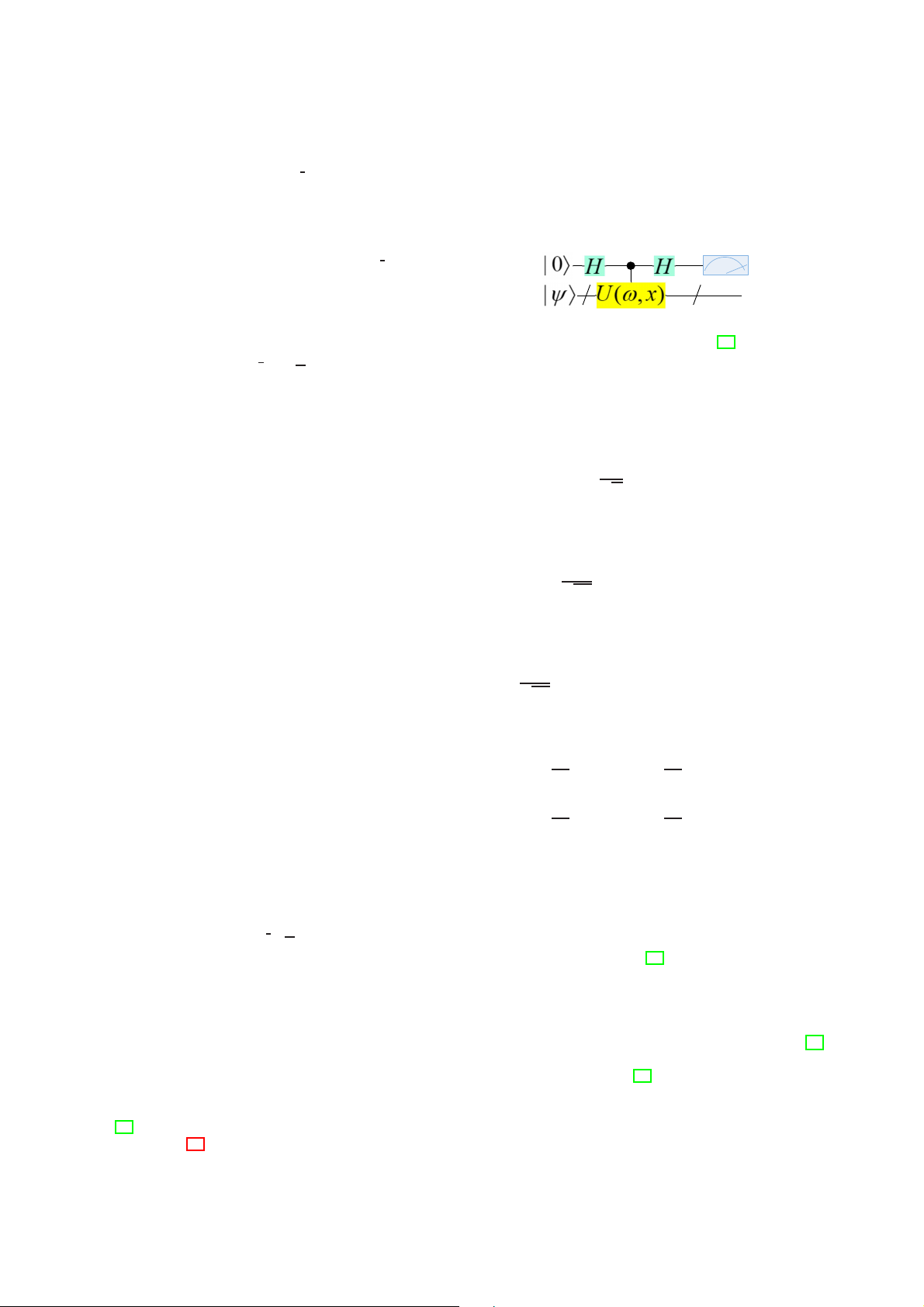
Fig. 16: The proposed QNN with 1-output and n-input called.
parameters, modified from [47].
In the second step, the quantum register is used to calculate
the inner product between i and w. By defining the unitary
In this circuit with 1-output and n-input parameters, |ψ→
transformation Uw and rotating the weighted quantum state to
will be initialized to an equal superposition state, so that the U
system qubit has an equal effect on the first qubit that produces
w|ψw→ = |1→⊗N = |m − 1→ (12)
the output. In the beginning, the initial input of the circuit is
, the task can be performed effectively. Any m × m unitary determined by matrix with ¯
wT in the last row meets this condition. If Uw is N added after U 1
i, the overall N-qubit quantum state becomes
|0→|ψ→ = √ |0→∑|j→, with N = kn (16) N m−1 j
Uw|ψi→ = ∑ cj| j→ ≡ |φi,w→ (13)
where |j→ is the jth vector in the standard basis. Hadamard j=0
gate and controlled U (ω, x) are applied to the first qubit, and
According to (12), the scalar product between two quantum the state becomes states is 1 N N $ψw | ψi→ = $ψw|U† ( eiαj wUw|ψi→ √ |0→∑|j→ + |1→∑ |j→) (17) (14) 2N = $ i i m − 1 | φi,w→ = cm−1
The parameter α j represents the phase value of the j-th
According to the definition of (10), the scalar product of
eigenvalue of U . After passing through the second Hadamard
the input vector and the weight vector is ¯ w, ¯i = m$ψw | ψi→.
gate, the final state is read as follows:
Therefore, the desired result is contained in the coefficient N N c 1
m−1 of the final state |φi,w→, which reaches a normalization √
(|0→∑(1 + eiαj)|j→ + |1→∑(1 − eiαj)|j→) (18) factor. 2N i i
To extract such information, an ancilla qubit (a) initially set
If the first qubit is measured, the probability of |0→ and |1→
to state |0→ is used. There is a multi-control NOT gate between
being P0 and P1 can be obtained from (18) as
the N-coded qubit and target a leading to 1 1 N m−2 P0 = ∑|1 + eiαj|2 = ∑(1 + cos(αj)) (19) |φ 4N 2N
i,w→|0→a → ∑ c j| j→|0→a + cm−1|m − 1→|1→a (15) j j j=0 1 1 N
The required nonlinearity of the threshold function of the P1 = ∑|1 − eiαj|2 = ∑(1 − cos(αj)) (20) 4N 2N
perceptron output is obtained immediately by performing a j j
quantum measurement. Measuring the state of ancilla qubits on
If a threshold function is applied to the output, then
the basis of the calculation produces output |0→a (i.e., an active !0 if P1 ≤ P0
perceptron) with probability |cm−1|2. It is important to note z = (21) 1 if P
that once the inner product information is stored on ancilla, 1 > P0
fine threshold functions can be applied. We also note that
After multiple measurements, z is described as the success
both parallel and antiparallel i − w vectors produce perceptron
probability of the expected output, that is, z = Pd.
activation, while orthogonal vectors always cause ancilla to be
The advantage of model of [47] is that a deviation term can measured in the |0→a state.
be added on this basis to adjust the threshold of the model.
This method has been experimentally verified on the IBM
In addition, the multi-input generalization ability of the model
quantum computer, and has taken a solid step from theory to
can have a variety of means, for example, the network can be
practice. However, subject to limited input qubits, the situation
generalized by sequentially applying Ujs.
with multiple qubits is not clear. In addition, as the number of
Since QP is a discrete binary input in many cases, [48]
input bits increases, the demand for quantum gates is getting
expands the input to a continuous input mode. In order to con-
higher and higher, which may cause unpredictable problems.
struct a more complex QP, [49] designs a Multi-Dimensional
In addition to neuron models, a large number of perceptron
Input QP (MDIQP) and implemented it by using ancilla qubit
models have also been proposed in recent years.
input control changes combined with phase estimation and
[47] proposed a simple QNN with periodic activation func-
learning algorithms. MDIQP can process quantum information
tion (see Fig. 16), which only requires O(n log2 n) qubits
and classify multi-dimensional data that may not be linearly. TE-2020-000227 11 H. Others
QWLNN architecture learning algorithm based on quantum
superposition. The architecture and parameters of this model
QCPNN D. Ventura introduces the idea of competitive
depend on many factors such as the number of training modes,
learning in QNN, and proposes a quantum competitive learn-
the structure of the selector, etc.
ing system based on Hamming distance metric [50]. The
competitive learning network completes the classification task
by comparing the input pattern and the pattern prototype IV. CHALLENGES AND OUTLOOK
encoded in the network weight. The basic idea is to determine
At this stage, although large-scale general-purpose quantum
the prototype that is most similar to the input mode (according
computers have not yet been truly implemented, the recent
to some indicators), and the class associated with the prototype
maturity of quantum processor technology has provided con-
is output as the class of the input mode. Based on the classic
ditions for simple verification of various quantum algorithms.
Hamming neural network algorithm, [51] incorporates quan-
In recent years, benefiting from commercial quantum com-
tum theory to obtain a new quantum Hamming neural network
puters developed by companies such as IBM, researchers can
based on competitive thinking. This kind of network does not
remotely manipulate dozens of qubits through the Internet,
rely on a complete model. Even if the pattern is incomplete, it
build simple quantum circuits, and realize small-scale quantum
can still be effectively trained, thereby increasing the probabil-
network systems. On the one hand, it provides a simple
ity of pattern recognition. And these unneeded patterns can be
experimental verification platform for various QNN models
further employed as new models for computational training.
and learning algorithms. On the other hand, it also regulates a
[52] uses the entanglement measure after the unitary operator
strict system framework for QNN theory research, that is, the
to compete between neurons to find the winner category on
QNN model and its learning algorithm must be oriented to real the basis of winner-takes-all.
quantum circuits and be strictly designed under the quantum
QSONN SONN is an artificial neural network that adopts
mechanics system. In this sense, the research work of QNN
an unsupervised competitive learning mechanism. It discovers
still has a long way to go, and the following key scientific
the internal laws of the input data by adjusting the network
issues urgently require further research.
parameters and structure through self-organization. [53] earlier
proposes a quantum version of SONN, which can perform
self-organizing and automatic pattern classification, without A. Linear and non-linear
the need for a dotted line to store the given pattern, and by
Activation function (such as sigmoid or tanh function),
modifying the value of the quantum register corresponding to
one of core elements in neural networks, has nonlinear char-
the classification. In order to enhance the clustering ability
acteristics. Its existence makes collective dynamics present
of QSONN, [54] projects the cluster samples and weights
dissipative characteristics and attractor-based, and makes it
from the competitive layer to the qubits on the Bloch sphere.
easier for neural networks to capture highly non-trivial patterns
The winning node can be known by calculating the spherical
[61]-[63]. But this is also the point of divergence from the
distance from the sample to the weight. Finally, the samples
linear unitary dynamics of quantum computing. Therefore, one
on the Bloch sphere are updated iteratively according to the
core question of QNN is whether it is possible to design a
weight values of the winning node and its neighborhood
framework to unify the non-linear dynamics of CNN with the
until convergence. In addition, following the classic parallel unitary dynamics of QNN
bidirectional self-organizing neural network, [55] proposes its
In order to solve this problem, the following suggestions quantum version.
can be used for reference: (1) Use simple dissipative quantum
CELL [56] introduces the CELL model in 1996. This
gates. (2) Explore the connection between quantum measure-
model is constructed using coupled quantum dot cells in
ments and activation functions. (3) Using quantum circuits to
an architecture instead of copying Boolean logic and using
approximate or fit nonlinear functions.
physical neighbor connections [56]. In the proposal of [57],
Dissipative quantum gates [26] introduces a nonlinear,
the quantum cellular automaton is regarded as the core neuron
irreversible, and dissipative operator. This operator can be
cell, and the two-layer quantum cellular automata array forms
intuitively regarded as a contraction operator, evolving the
a three-dimensional CELL which has the structure of A clone
general state into a single (stable) state, and the nonlinearity
template, B clone template and threshold. And the validity
depends only on its amplitude and not on the phase. When
of its model is proved in image processing. [58] proposes a
designing a QNN, there is an irreversible operator behind the
fractional-order image encryption CELL model, which uses
reversible unitary operator. This method has a certain degree
deformed fractional Fourier transform to solve the problem of
of feasibility from a theoretical point of view, but it is very
insufficient non-linearity. The specific principle is as follows:
difficult at the level of implementation.
the input image is processed by the first chaotic random phase
Quantum measurements [64] designs a QNN model based
mask, and then processed by the first chaotic random phase
on quantum measurement, which attempts to integrate the
mask. Finally, the encrypted image is generated in the second
reversible unitary structure of quantum evolution with the
chaotic random phase mask as well as the second deformed
irreversible nonlinear dynamics of neural networks. The au-
fractional Fourier transform in sequence. The cryptographic
thor uses an open quantum walk to try to replace the step
system shows strong resistance to a variety of potential attacks.
function or the sigmoid activation function through quantum
QWLNN [59] mentions QWLNN in 2008. [60] defines a
measurement, and find a quantum form to capture the two TE-2020-000227 12
main characteristics of the Hopfield network, dissipation and
select the remaining ones. Such circuits constitute a sequence nonlinearity.
of shallow blocks, and each shallow block calculates the
Quantum circuits The interpretation of nonlinear activation
identity, which controls the effective depth of the circuit for a
functions by quantum circuits is currently a popular practice.
parameter update, so that they will not enter the barren plateau
Especially the application of RUS technology to solve the at the beginning of training.
problem of nonlinear activation function [20][65]-[67].
The above references are only a useful attempt on the barren
plateau, but the problem of the barren plateau has not been
B. Verification of quantum superiority
solved perfectly and is a problem worthy of study.
Limited by the current level of quantum computing hard- A
ware, QNN can only perform experiments on low-dimensional CKNOWLEDGMENT
and small sample problems, and it is difficult to verify its
We would like to thank all the reviewers who provided
advantages over CNN. In response to this key issue, it is nec-
valuable suggestions and Chen Zhaoyun, Ph.D., Department
essary to establish a unified quantitative index and calculation
of Physics, University of Science and Technology of China.
model to accurately compare the operating complexity and
resource requirements of QNN and CNN and to strictly prove REFERENCES
the superiority of quantum computing compared to classical
[1] R. P. Feynman, “Simulating physics with computers,” International
computing. In addition, it is necessary to strictly verify the
Journal of Theoretical Physics, vol. 21, no. 6, pp. 467-488, 1982.
prediction accuracy and generalization performance of the
[2] F. Arute et al., ”Quantum supremacy using a programmable supercon-
ducting processor,” Nature, vol. 574, no. 7779, pp. 505-510, 2019/10/01
QNN on a large benchmark data set. At present, there are few 2019.
related studies. [68] and [69] have made an in-depth discussion
[3] E. Pednault, J. Gunnels, D. Maslov, and J. Gambetta, “On quantum
on the superiority of quantum optimization algorithms for
supremacy,” IBM Research Blog, vol. 21, 2019.
[4] J. Preskill, “Quantum computing in the NISQ era and beyond,” Quan-
recent quantum processors compared to classical optimization tum, vol. 2, pp. 79, 2018.
algorithms. Perhaps we can be inspired by them.
[5] S. C. Kak, ”Quantum Neural Computing,” Advances in Imaging and
Electron Physics, P. W. Hawkes, ed., pp. 259-313: Elsevier, 1995.
[6] R. Parthasarathy and R. Bhowmik, ”Quantum Optical Convolutional C. Barren plateau
Neural Network: A Novel Image Recognition Framework for Quantum
Computing,” IEEE Access, pp. 1-1, 2021.
What the Barren Plateau wants to express is that when the
[7] D. Yumin, M. Wu, and J. Zhang, ”Recognition of Pneumonia Image
amount of qubits is comparatively large, the current QNN
Based on Improved Quantum Neural Network,” IEEE Access, vol. 8,
framework is easily changed and cannot be effectively trained, pp. 224500-224512, 2020.
[8] G. Liu, W.-P. Ma, H. Cao, and L.-D. Lyu, ”A quantum Hopfield neural
that is, the objective function will become very flat, making the
network model and image recognition,” Laser Physics Letters, vol. 17,
gradient difficult to estimate [70]. The root cause of this phe-
no. 4, p. 045201, 2020/02/27 2020.
nomenon is: according to the objective function constructed
[9] L. Fu, and J. Dai, ”A Speech Recognition Based on Quantum Neural
Networks Trained by IPSO.” pp. 477-481, 2009.
by the current quantum circuit (satisfying t-design), the mean
[10] C. H. H. Yang et al., ”Decentralizing Feature Extraction with Quantum
value of the gradient of the circuit parameters (some rotation
Convolutional Neural Network for Automatic Speech Recognition,” in
angles) is 0. And the variance exponentially decreases as the
ICASSP 2021 - 2021 IEEE International Conference on Acoustics,
Speech and Signal Processing (ICASSP), 6-11 June 2021 2021.
total of qubits increases [70].
[11] P. Kairon, and S. Bhattacharyya, ”COVID-19 Outbreak Prediction Using
[71] extends the Barren Plateau Theorem from a single
Quantum Neural Networks,” Intelligence Enabled Research: DoSIER
2-design circuit to any parameterized quantum circuit, and
2020, S. Bhattacharyya, P. Dutta and K. Datta, eds., pp. 113-123,
Singapore: Springer Singapore, 2021.
gives reasonable presumptions so that certain integrals can
[12] E. El-shafeiy, A.-E. Hassanien, K.-M. Sallam et al., “Approach for
be expressed as ZX-graphs and calculated using ZX-calculus.
Training Quantum Neural Network to Predict Severity of COVID-19
The results show that there is a barren plateau for hardware-
in Patients,” Computers, Materials & Continua, vol. 66, no. 2, pp. 1745- 1755, 2021.
efficient ansatz and ansatz inspired by MPS, while for QCVNN
[13] A. A. Ezhov, and D. Ventura, ”Quantum Neural Networks,” Future
ansatz and tree tensor network ansatz, there is no barren
Directions for Intelligent Systems and Information Sciences: The Future plateau [71].
of Speech and Image Technologies, Brain Computers, WWW, and
Bioinformatics, N. Kasabov, ed., pp. 213-235, Heidelberg: Physica-
VQA is a commonly useful method of constructing QNN, Verlag HD, 2000.
which optimizes the parameters θ through the parameterized
[14] V. Raul, T. Beatriz, and M. Hamed, ”A Quantum NeuroIS Data Analytics
quantum circuit V (θ ), with the purpose of minimizing the
Architecture for the Usability Evaluation of Learning Management
Systems,” Quantum-Inspired Intelligent Systems for Multimedia Data
cost function C. Considering the connection between it and
Analysis, B. Siddhartha, ed., pp. 277-299, Hershey, PA, USA: IGI
the barren plateau, [72] points out that even if V (θ ) is very Global, 2018.
shallow, defining C with a globally observable value will result
[15] J. R. McClean, J. Romero, R. Babbush et al., “The theory of variational
hybrid quantum-classical algorithms,” New Journal of Physics, vol. 18,
in a barren plateau. However, as long as the depth of V (θ ) is
no. 2, pp. 023023, 2016/02/04, 2016.
O(log n), defining C with a locally observable value will lead
[16] A. Abbas, D. Sutter, C. Zoufal et al., “The power of quantum neural
to a polynomial vanishing gradient in the worst case, thus
networks,” Nature Computational Science, vol. 1, no. 6, pp. 403-409, 2021/06/01, 2021.
establishing a connection between locality and trainability.
[17] J. Zhao, Y.-H. Zhang, C.-P. Shao et al., “Building quantum neural
In order to solve the problem of the barren plateau, it
networks based on a swap test,” Physical Review A, vol. 100, no. 1,
seems to be a good choice to cut from the perspective of pp. 012334, 07/23/, 2019.
[18] P. Li, and B. Wang, “Quantum neural networks model based on swap
initialization. In the scheme proposed by [73], the first step
test and phase estimation,” Neural Networks, vol. 130, pp. 152-164,
is to randomly select some initial parameter values, and then 2020/10/01/, 2020. TE-2020-000227 13
[19] H. Buhrman, R. Cleve, J. Watrous et al., “Quantum Fingerprinting,”
[49] A. Y. Yamamoto, K. M. Sundqvist, P. Li, and H. R. Harris, “Simulation
Physical Review Letters, vol. 87, no. 16, pp. 167902, 09/26/, 2001.
of a Multidimensional Input Quantum Perceptron,” Quantum Informa-
[20] Y. Cao, G. G. Guerreschi, and A. Aspuru-Guzik, “Quantum neuron: an
tion Processing, vol. 17, no. 6, Jun, 2018.
elementary building block for machine learning on quantum computers,”
[50] D. Ventura, ”Implementing competitive learning in a quantum system.”
arXiv preprint arXiv:1711.11240, 2017. pp. 462-466 vol.1, 1999.
[21] A. Paetznick, and K. Svore, “Repeat-until-success: non-deterministic
[51] M. Zidan, A. Sagheer, and N. Metwally, ”An autonomous competitive
decomposition of single-qubit unitaries,” Quantum Inf. Comput., vol.
learning algorithm using quantum hamming neural networks.” pp. 1-7, 14, pp. 1277-1301, 2014. 2015.
[22] K. H. Wan, O. Dahlsten, H. Kristjansson et al., “Quantum generalisation
[52] M. Zidan, A.-H. Abdel-Aty, M. El-shafei, M. Feraig, Y. Al-Sbou, H.
of feedforward neural networks,” NPJ QUANTUM INFORMATION,
Eleuch, and M. Abdel-Aty, “Quantum Classification Algorithm Based vol. 3, SEP 14, 2017.
on Competitive Learning Neural Network and Entanglement Measure,”
[23] M. Schuld, I. Sinayskiy, and F. Petruccione, “The quest for a Quantum
Applied Sciences, vol. 9, no. 7, 2019.
Neural Network,” Quantum Information Processing, vol. 13, no. 11, pp.
[53] Z. Rigui, Z. Hongyuan, J. Nan, and D. Qiulin, ”Self-Organizing Quan- 2567-2586, 2014/11/01, 2014.
tum Neural Network.” pp. 1067-1072, 2006.
[24] T. Menneer, and A. Narayanan, “Quantum-inspired neural networks,”
[54] Z. Li, and P. Li, “Clustering algorithm of quantum self-organization Tech. Rep. R329, 1995.
network,” Open Journal of Applied Sciences, vol. 5, no. 06, pp. 270,
[25] E. C. Behrman, L. Nash, J. E. Steck et al., “Simulations of quantum 2015.
neural networks,” Information Sciences, vol. 128, no. 3-4, pp. 257-269,
[55] D. Konar, S. Bhattacharyya, B. K. Panigrahi, and M. K. Ghose, ”Chapter 2000.
5 - An efficient pure color image denoising using quantum parallel bidi-
[26] S. Gupta, and R. K. P. Zia, “Quantum Neural Networks,” Journal of
rectional self-organizing neural network architecture,” Quantum Inspired
Computer and System Sciences, vol. 63, no. 3, pp. 355-383, 2001/11/01/,
Computational Intelligence, S. Bhattacharyya, U. Maulik and P. Dutta, 2001.
eds., pp. 149-205, Boston: Morgan Kaufmann, 2017. [27] M. V. Altaisky, “Quantum neural network,” arXiv preprint
[56] G. Toth, C. S. Lent, P. D. Tougaw, Y. Brazhnik, W. Weng, W. Porod, quant-ph/0107012, 2001.
R.-W. Liu, and Y.-F. Huang, “Quantum cellular neural networks,” Su-
[28] N. Killoran, T. R. Bromley, J. M. Arrazola et al., “Continuous-variable
perlattices and Microstructures, vol. 20, no. 4, pp. 473-478, 1996/12/01/,
quantum neural networks,” Physical Review Research, vol. 1, no. 3, pp. 1996. 033063, 10/31/, 2019.
[57] S. Wang, L. Cai, H. Cui, C. Feng, and X. Yang, ”Three-dimensional
[29] P. Zhang, S. Li, and Y. Zhou, “An Algorithm of Quantum Restricted
quantum cellular neural network and its application to image process-
Boltzmann Machine Network Based on Quantum Gates and Its Appli- ing.” pp. 411-415, 2017.
cation,” Shock and Vibration, vol. 2015, pp. 756969, 2015/09/15, 2015.
[58] X. Liu, X. Jin, and Y. Zhao, ”Optical Image Encryption Using
[30] Y. Shingu, Y. Seki, S. Watabe et al., “Boltzmann machine learning with a
Fractional-Order Quantum Cellular Neural Networks in a Fractional
variational quantum algorithm,” arXiv preprint arXiv:2007.00876, 2020.
Fourier Domain.” pp. 146-154, 2018.
[31] C. Zoufal, A. Lucchi, and S. Woerner, “Variational quantum Boltz-
[59] W. R. d. Oliveira, A. J. Silva, T. B. Ludermir, A. Leonel, W. R. Galindo,
mann machines,” Quantum Machine Intelligence, vol. 3, no. 1, pp. 7,
and J. C. C. Pereira, ”Quantum Logical Neural Networks.” pp. 147-152, 2021/02/22, 2021. 2008.
[32] G. Chen, Y. Liu, J. Cao et al., ”Learning Music Emotions via Quantum
[60] A. J. da Silva, W. R. de Oliveira, and T. B. Ludermir, “Weightless neural
Convolutional Neural Network,” Brain Informatics. pp. 49-58, 2017.
network parameters and architecture selection in a quantum computer,”
[33] I. Cong, S. Choi, and M. D. Lukin, “Quantum convolutional neural
Neurocomputing, vol. 183, pp. 13-22, 2016/03/26/, 2016.
networks,” Nature Physics, vol. 15, no. 12, pp. 1273-1278, 2019/12/01,
[61] M. I. Rabinovich, P. Varona, A. I. Selverston, and H. D. I. Abarbanel, 2019.
“Dynamical principles in neuroscience,” Reviews of Modern Physics,
[34] Y. Li, R.-G. Zhou, R. Xu et al., “A quantum deep convolutional neural
vol. 78, no. 4, pp. 1213-1265, 11/14/, 2006.
network for image recognition,” Quantum Science and Technology, vol.
5, no. 4, pp. 044003, 2020/07/20, 2020.
[62] J. J. Hopfield, “Neural networks and physical systems with emergent
collective computational abilities,” Proceedings of the National Academy
[35] S. Lloyd, and C. Weedbrook, “Quantum Generative Adversarial Learn-
of Sciences, vol. 79, no. 8, pp. 2554, 1982.
ing,” Physical Review Letters, vol. 121, no. 4, pp. 040502, 07/26/, 2018.
[36] P.-L. Dallaire-Demers, and N. Killoran, “Quantum generative adversarial
[63] G. E. Hinton, and R. R. Salakhutdinov, “Reducing the Dimensionality
networks,” Physical Review A, vol. 98, no. 1, pp. 012324, 07/23/, 2018.
of Data with Neural Networks,” Science, vol. 313, no. 5786, pp. 504,
[37] L. Bai, Y. Jiao, L. Rossi et al., “Graph Convolutional Neural Networks 2006.
based on Quantum Vertex Saliency,” arXiv preprint arXiv:1809.01090,
[64] M. Zak, and C. P. Williams, “Quantum Neural Nets,” International 2018.
Journal of Theoretical Physics, vol. 37, no. 2, pp. 651-684, 1998/02/01,
[38] S. Dernbach, A. Mohseni-Kabir, S. Pal et al., ”Quantum Walk Neural 1998.
Networks for Graph-Structured Data,” Complex Networks and Their
[65] W. Hu, “Towards a real quantum neuron,” Natural Science, vol. 10, no. Applications VII. pp. 182-193. 3, pp. 99-109, 2018.
[39] J. Zheng, Q. Gao, and Y. Lv, “Quantum Graph Convolutional Neural
[66] F. M. d. P. Neto, T. B. Ludermir, W. R. d. Oliveira, and A. J. d. Silva,
Networks,” arXiv preprint arXiv:2107.03257, 2021.
“Implementing Any Nonlinear Quantum Neuron,” IEEE Transactions on
[40] Y. Takaki, K. Mitarai, M. Negoro et al., “Learning temporal data with a
Neural Networks and Learning Systems, vol. 31, no. 9, pp. 3741-3746,
variational quantum recurrent neural network,” Physical Review A, vol. 2020. 103, no. 5, pp. 052414, 2021.
[67] S. Yan, H. Qi, and W. Cui, “Nonlinear quantum neuron: A fundamental
[41] J. Bausch, “Recurrent quantum neural networks,” arXiv preprint
building block for quantum neural networks,” Physical Review A, vol. arXiv:2006.14619, 2020. 102, no. 5, pp. 052421, 2020.
[42] W. Huggins, P. Patil, B. Mitchell et al., “Towards quantum machine
[68] E. Farhi, and A. W. Harrow, “Quantum supremacy through the quantum
learning with tensor networks,” Quantum Science and Technology, vol.
approximate optimization algorithm,” arXiv preprint arXiv:1602.07674,
4, no. 2, pp. 024001, 2019/01/09, 2019. 2016.
[43] L. Fei, and Z. Baoyu, ”A study of quantum neural networks.” pp. 539-
[69] L. Zhou, S.-T. Wang, S. Choi, H. Pichler, and M. D. Lukin, “Quantum 542, 2003.
Approximate Optimization Algorithm: Performance, Mechanism, and
[44] L. Fei, Z. Shengmei, and Z. Baoyu, ”Feedback Quantum Neuron and
Implementation on Near-Term Devices,” Physical Review X, vol. 10,
Its Application.” pp. 867-871, 2005.
no. 2, pp. 021067, 06/24/, 2020.
[45] L. B. Kristensen, M. Degroote, P. Wittek et al., “An artificial spiking
[70] J. R. McClean, S. Boixo, V. N. Smelyanskiy, R. Babbush, and H. Neven,
quantum neuron,” npj Quantum Information, vol. 7, no. 1, pp. 1-7, 2021.
“Barren plateaus in quantum neural network training landscapes,” Nature
[46] F. Tacchino, C. Macchiavello, D. Gerace et al., “An artificial neuron im-
Communications, vol. 9, no. 1, pp. 4812, 2018/11/16, 2018.
plemented on an actual quantum processor,” npj Quantum Information,
[71] C. Zhao, and X. Gao, “Analyzing the barren plateau phenomenon in vol. 5, no. 1, pp. 1-8, 2019.
training quantum neural network with the ZX-calculus,” Quantum, vol.
[47] A. Daskin, ”A Simple Quantum Neural Net with a Periodic Activation 5, pp. 466, 2021.
Function.” pp. 2887-2891, 2018.
[72] M. Cerezo, A. Sone, T. Volkoff, L. Cincio, and P. J. Coles, “Cost function
[48] M. Maronese, and E. Prati, “A continuous rosenblatt quantum percep-
dependent barren plateaus in shallow parametrized quantum circuits,”
tron,” International Journal of Quantum Information, pp. 2140002, 2021.
Nature Communications, vol. 12, no. 1, pp. 1791, 2021/03/19, 2021. TE-2020-000227 14
[73] E. Grant, L. Wossnig, M. Ostaszewski, and M. Benedetti, “An initial-
ization strategy for addressing barren plateaus in parametrized quantum
circuits,” Quantum, vol. 3, pp. 214, 2019.