Chapter 2 - Graphical Method & Problem Formulation Notes | Môn Deterministic Models in Operations Research - Trường Đại học Quốc tế, Đại học Quốc gia Thành phố Hồ Chí Minh

lOMoAR cPSD| 58583460 Chapter 2: Linear Programming Introduction about LP Problem Formulation
Solve LP using Graphical approach Four Special Cases Sensitivity Analysis
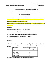
Notes: From now on, in every lecture, all students must
participate into the activities of the class. The results of
these activities will be scored and allocated to the
assigments/homeworks at the end of the semester. lOMoAR cPSD| 58583460 1. Introduction
Many decisions in management are related
with the best usage resources of organizations.
Manager makes Decisions in order to satisfy
Objectives, Goals of organizations.
Resources: Materials, Machines, Man, Money, Time, Space.
Linear Programming (LP) is a mathematical
method that helps managers to make decision related with lOMoAR cPSD| 58583460
Resources Allocation. (references about Nobel laureate: Kantorovich) Extensively using computer. 3 LP PROBLEM
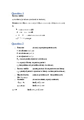
Problem: determine some variables to
Maximize or Minimize, usually Profit/ Cost,
called Objective function.
Constraints: are functions show resources
limitation of companies/ organizations. The
problem is to find s solution that maximize lOMoAR cPSD| 58583460
profits (or minimize lost/cost) in given constraints.
Form of constraint functions could be: Inequality (form or ) Equality 4
All Objective function and Constraint
functions are linear functions. An Example of an LP model
ABC company manufactures two products: Item A and Item B Each Item A:
Sell for $27 and uses $19 worth of raw materials. lOMoAR cPSD| 58583460
Increase ABC’s variable labor/overhead costs by $5.
Requires 2 hours of finishing labor. Requires 1 hour of carpentry labor. Each Item B:
Sell for $21 and used $9 worth of raw materials.
Increases ABC’s variable labor/overhead costs by $10.
Requires 1 hour of finishing labor.
Requires 1 hour of carpentry labor. Each week ABC can obtain:
All needed raw material. Only 100 finishing hours. Only 80 carpentry hours.
Demand for the Item B is unlimited.
At most 40 Item A are bought each week.
ABC wants to maximize weekly profit (revenues – costs). ABC’s LP model
x1 = number of item A produced each week
x2 = number of item B produced each week lOMoAR cPSD| 58583460 Max z = 3x1 + 2x2 (objective function)
(Weekly profit = weekly revenue – weekly raw material costs – the weekly variable
costs = 3x1 + 2x2) Subject to (s.t.)
Each week, no more than 100 hours of finishing time may be used.
2 x1 + x2 ≤ 100 (finishing constraint)
Each week, no more than 80 hours of carpentry time may be used. (x1 + x2 ≤ 80) x1 + x2 ≤ 80 (carpentry constraint)
Because of limited demand, at most 40 item A should be produced. (x1 ≤ 40)
x1 ≤ 40 (constraint on demand for Item A) x1 ≥ 0
(sign restriction) x2 ≥ 0 (sign restriction) lOMoAR cPSD| 58583460 2. Formulating LP Problems WYNDOR GLASS CO.
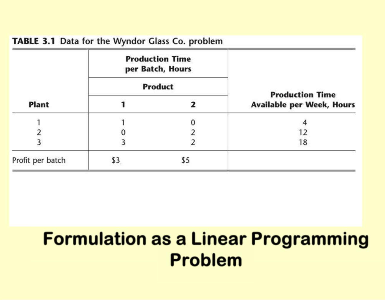
Glass products : windows and glass doors.
Plant 1: Aluminum frames and hardware : Product 1
Plant 2: Wood frame: Product 2
Plant 3: The glass and assembles the products: Product 1 & 2.
Product 1: An 8-foot glass door with aluminum framing lOMoAR cPSD| 58583460
Product 2: A 4x6 foot double-hung wood-framed window
WYNDOR GLASS CO problem: Determine what the production
rates should be for the two products in order to
maximize their total profit
The production rate = The number of batches of
the products to be produced / week WYNDOR GLASS CO Data lOMoAR cPSD| 58583460
Formulation as a Linear Programming Problem lOMoAR cPSD| 58583460
x1 = number of batches of product 1 produced per week
x2 = number of batches of product 2 produced per week
Z = total profit per week (in thousands of dollars) from producing these two products The objective function is Maximize profit Z = $3x1 + $5x2 Subject to the restrictions: 3x1 + 2x2 18 2x2 12 x1 4Linear Programming Problem x1 0 x2 0. lOMoAR cPSD| 58583460 3. Graphical Solution
The graphical method works only when there are
two decision variables, but it provides valuable
insight into how larger problems are structured
Graphical Representation of Constraints
• Isoprofit-line method
• Corner points method lOMoAR cPSD| 58583460
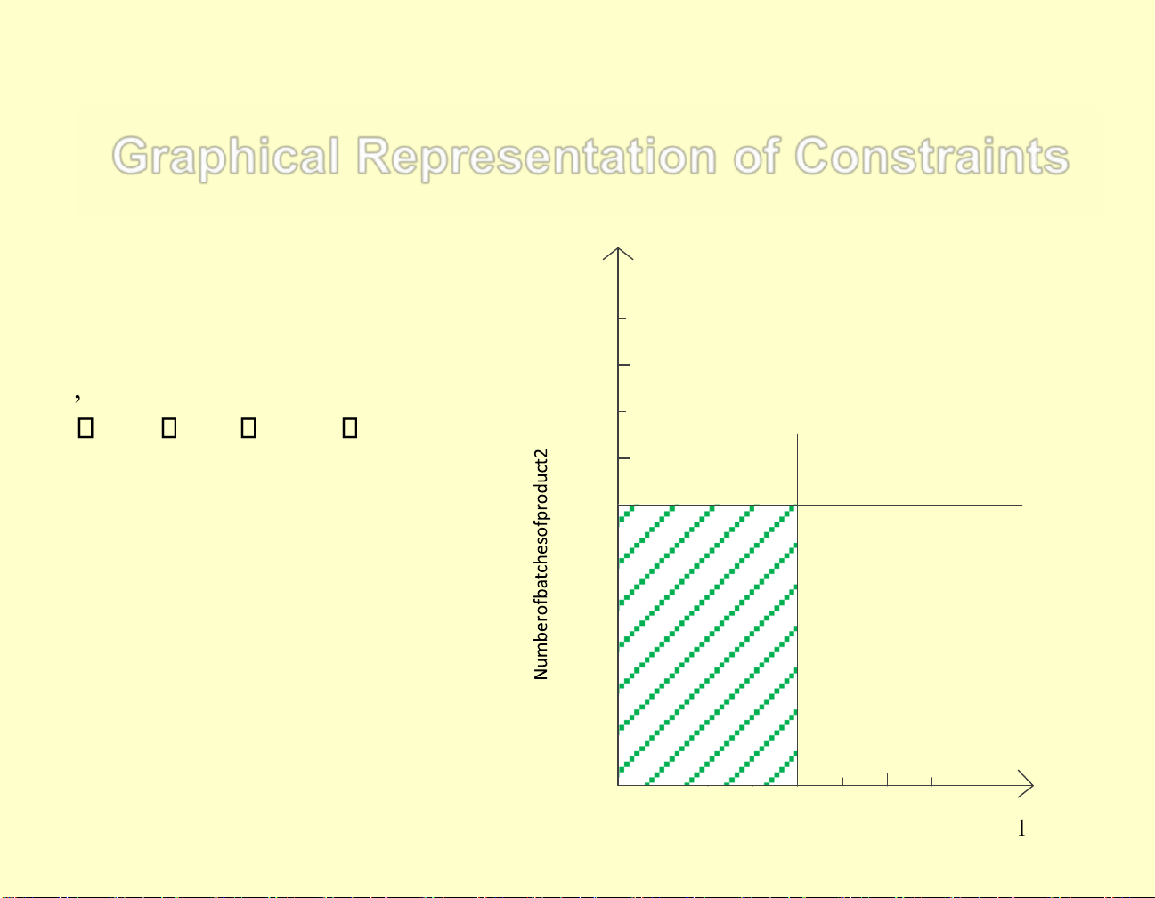
Graphical Representation of Constraints 2 x
Fig 1. Shaded area shows values of 9 ( 1 , xx 2 ) allowed by 8 x , 0 2 x , 0 1 x , 4 2 2 x 12 7 2 = 2 x 12 6 5 = 4 1 x 4 3 2 1 0 1 2 3 4 5 6 7 1 x 1 lOMoAR cPSD| 58583460
Number of batches of product 1 lOMoAR cPSD| 58583460
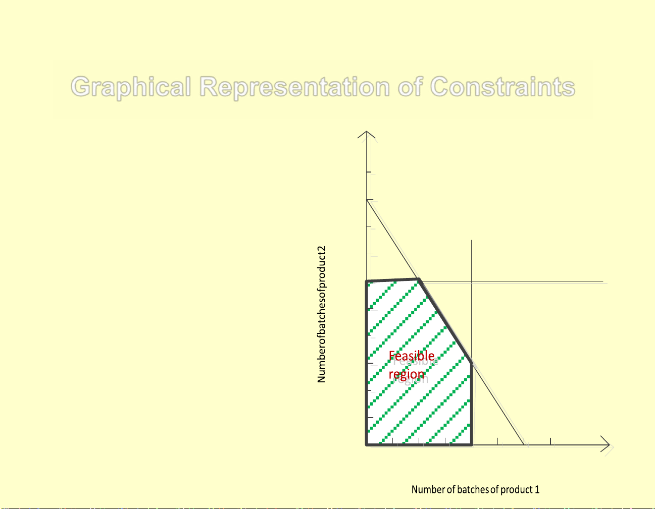
Graphical Representation of Constraints 2 x 9
Fig 2. Shaded area shows the set of 3 + = 1 x 2 x 18 2
permissible values of (x 1 , x 2 ) , called the 8 feasible region . 7 2 = 2 x 12 6 5 = 4 1 x 4 3 2 1 0 1 2 3 4 5 6 7 1 x lOMoAR cPSD| 58583460
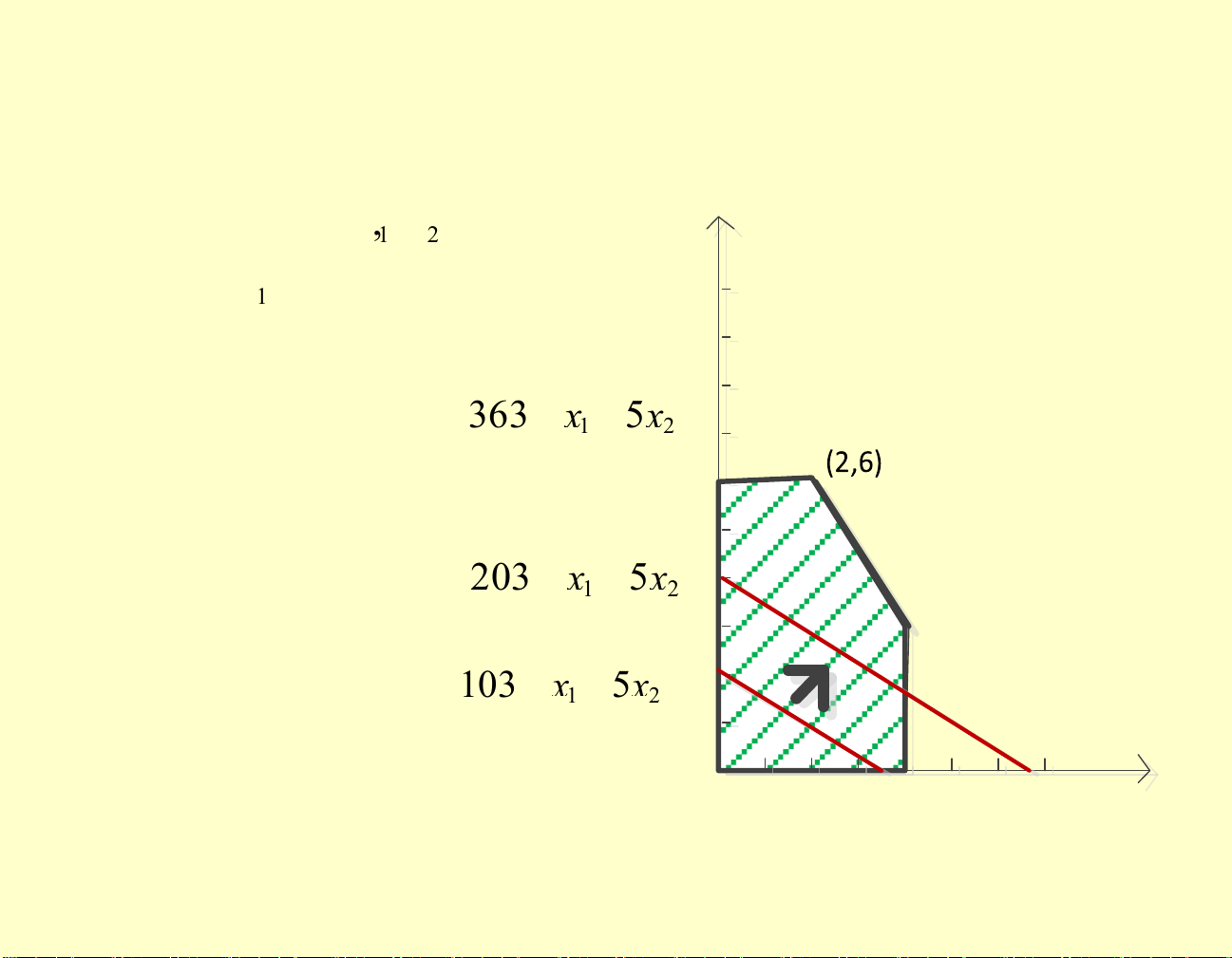
3.1. Isoprofit- line method Fig 3. The value 1 of (, xx ) that 2 2 x maximizes 3 + 1 x 5 x is (2, 2 6). 9 9 8 8 Z ==+ 363 1 x 5x 2 77 6 6 5 5 Z ==+ 203 1 x 5x 2 4 4 3 3 Z ==+ 2 103 1 x 5x 2 2 1 1 x 0 1 2 3 4 5 6 7 1 lOMoAR cPSD| 58583460
Solving LP graphically by Isoprofit- line method 3 1 x2
x2 =− x1 + Z Optimal solution 5 5 I == = ( 1 x , x 2 6) 2 0 1 2 3 4 5 6 7 1 x lOMoAR cPSD| 58583460 99 Z = = +36 3x 88 1 5x2 77 66 5 5
Z = = +20 3x1 5x2 4 4 Max Profit: Z=3*2+5*6=3 33
Z = = +10 3x1 5x2 22 11 lOMoAR cPSD| 58583460
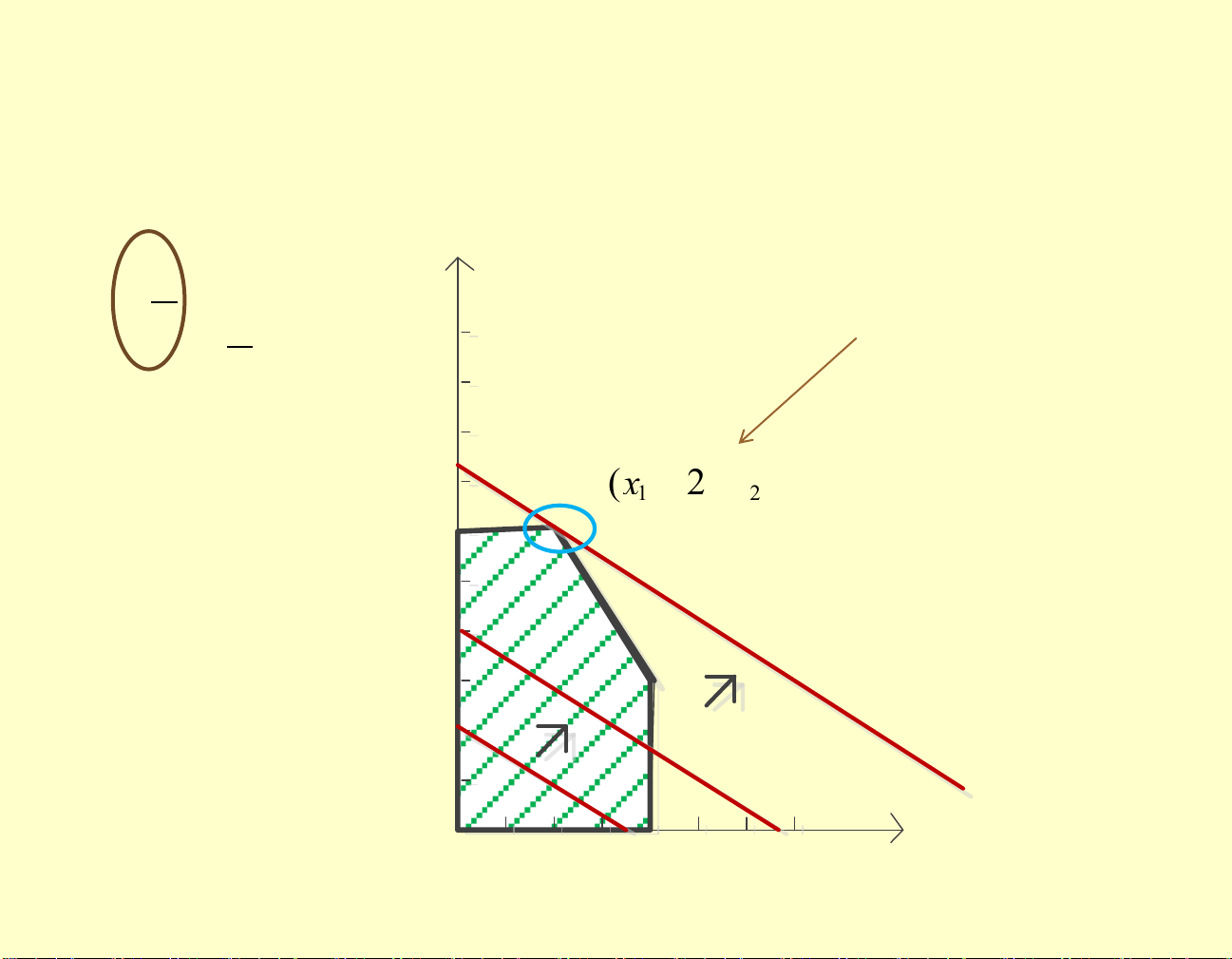
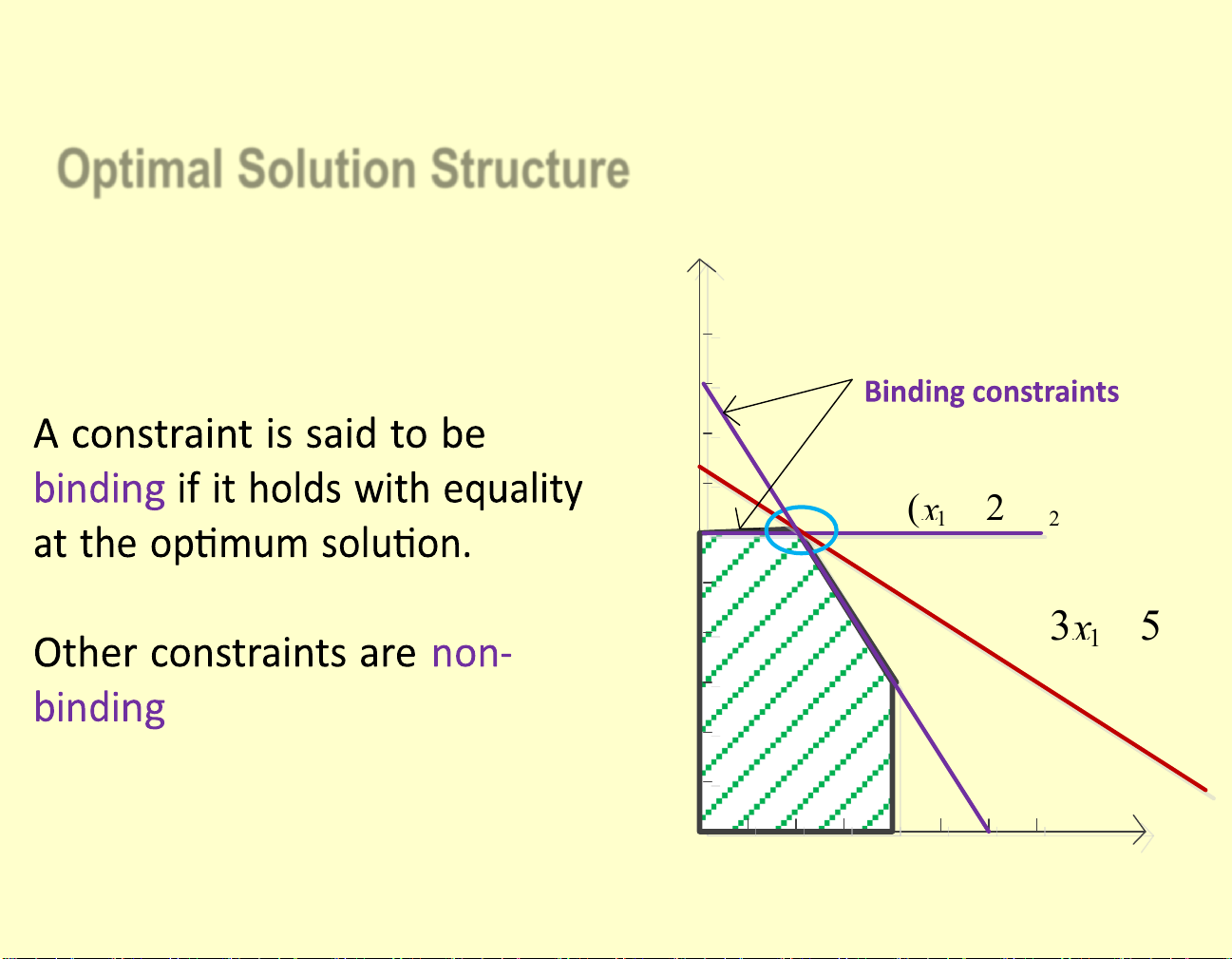
Optimal Solution Structure 2 x 9 9 8 8 7 7 I == = ( 1 x , x 2 6) 2 6 6 5 5 Z =+ 3 x 5x 4 4 1 2 3 3 2 2 1 1 0 1 2 3 4 5 6 7 1 x lOMoAR cPSD| 58583460 Remarks:
Isoprofit lines (Z): parallel (same slope).
Optimal solution (any points): intersected (touched) by
the feasible region and isoprofit line that defines the largest Z-value.
 Find the objective is to minimize Z: try Z-values tend to decrease
Find the objective is to maximize Z: try Z-values tend to increase lOMoAR cPSD| 58583460
3.2. Corner-point method
Objective: Maximize Profit Z = 3X1 +
5X2 The mathematical theory in LP shows
that the optimal solution must lie at one
corner point, or extreme point, of the feasible region • At A=(0,0): Profit = 0 • At B=(0,6):
Profit = 3(0) + 5(6) = 30 • At C=(2,6):