Chapter-5 - Math for business | Trường Đại học Quốc tế, Đại học Quốc gia Thành phố HCM

1 | M A T H F O R B U S I N E S S C H A P T E R 5 Chapter 5:
Partial Differentiation I.
Functions of several variables
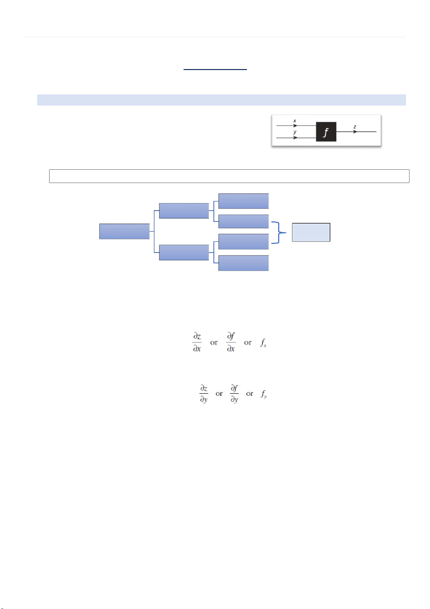
1. The function notation, z = f(x,y)
A rule that assigns to each incoming pair of numbers, (x, y),
a uniquely defined outgoing number, z .
2. The first and second order partial derivatives
Given a function of two variables, z = f (x, y) fxx fx fxy f (x,y) fxy = fyx fyx fy fyy 2.1.
The first – order partial derivatives -
We can determine two first-order derivatives. (Tìm partial derivative cÿa hàm số theo mßt
bi¿n nào đó, xem các bi¿n còn l¿i nh± HẰNG SỐ) -
The partial derivative of f with respect to x is written as
(found by differentiating f with respect to x, with y held constant) -
The partial derivative of f with respect to y is written as
(found by differentiating f with respect to x, with y held constant) 2.2.
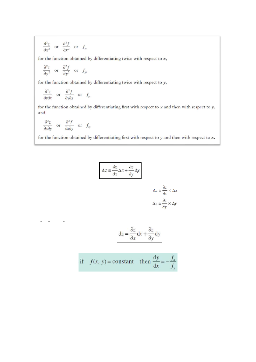
The second – order partial derivatives
Contact: ngominhtuyetngoc216@gmail.com
2 | M A T H F O R B U S I N E S S C H A P T E R 5
3. Young’s theorem: fxy = fyx
4. Use the small increments formula. Small increments formula:
(x and y both change simultaneously) Explain:
+ x changes by a small amount ∆ý and y is fixed:
+ y changes by a small amount ∆þ and x is fixed:
 dx , dy and dz (differentials): represent limiting values of Δx , Δy and Δz , respectively:
5. Perform implicit differentiation.
Contact: ngominhtuyetngoc216@gmail.com
3 | M A T H F O R B U S I N E S S C H A P T E R 5 EXERCISE (5.1)
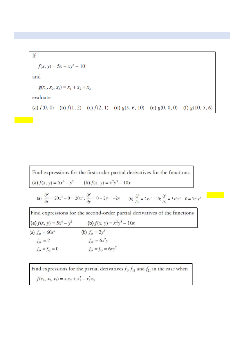
1. Use the function notation, z = f (x, y) Solution:
a) To evaluate the function f (x, y) = 5x + xy2 – 10, substitute the numerical values x = 0 and y = 0 gives:
f (0,0) = 5(0) + 0(02) – 10 = - 10 b) 21 c) 2 d) 21 e) 0 f)21
2. The 1st and 2nd order partial derivatives Solution:
3. Young’s theorem: fxy = fyx
Contact: ngominhtuyetngoc216@gmail.com
4 | M A T H F O R B U S I N E S S C H A P T E R 5 Solution:
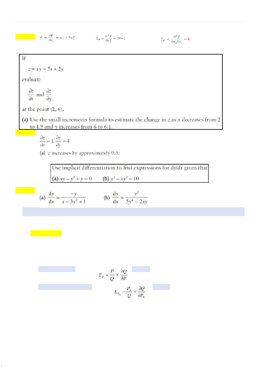
4. Use the small increments formula. Solution:
5. Perform implicit differentiation. Solution: II.
Partial elasticity and marginal functions
1. Calculate partial elasticities. Q = f(P, PA, Y)
When Q: demand for a certain good P: the good’s price
PA: the price of an alternative good Y: the income of consumers. - Price elasticity of demand: - Cross price elasticity of – demand: + Positive: substitutable
Contact: ngominhtuyetngoc216@gmail.com
5 | M A T H F O R B U S I N E S S C H A P T E R 5 + Negative: complementary - Income elasticity of demand:
+ Ey < 0 → inferior goods (white bread, instant noodle, bus transportation) + Ey > 0 • < 1: normal goods
• >1: superior goods (sport cars, quality wine, &)
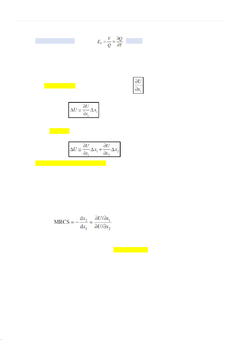
2. Calculate marginal utilities. - The marginal utility of xi
+ The rate of change of U with respect to xi
+ If xi changes by a small amount Δxi and the other variable is fixed then the change in U satisfies -
Suppose that there are two goods, G1 (the consumer buys x1 items) and G2 (x2).
+ U (utility) indicates the level of satisfaction.
+ If x1 and x2 both change then the net change in U can be found from the small increments formula -
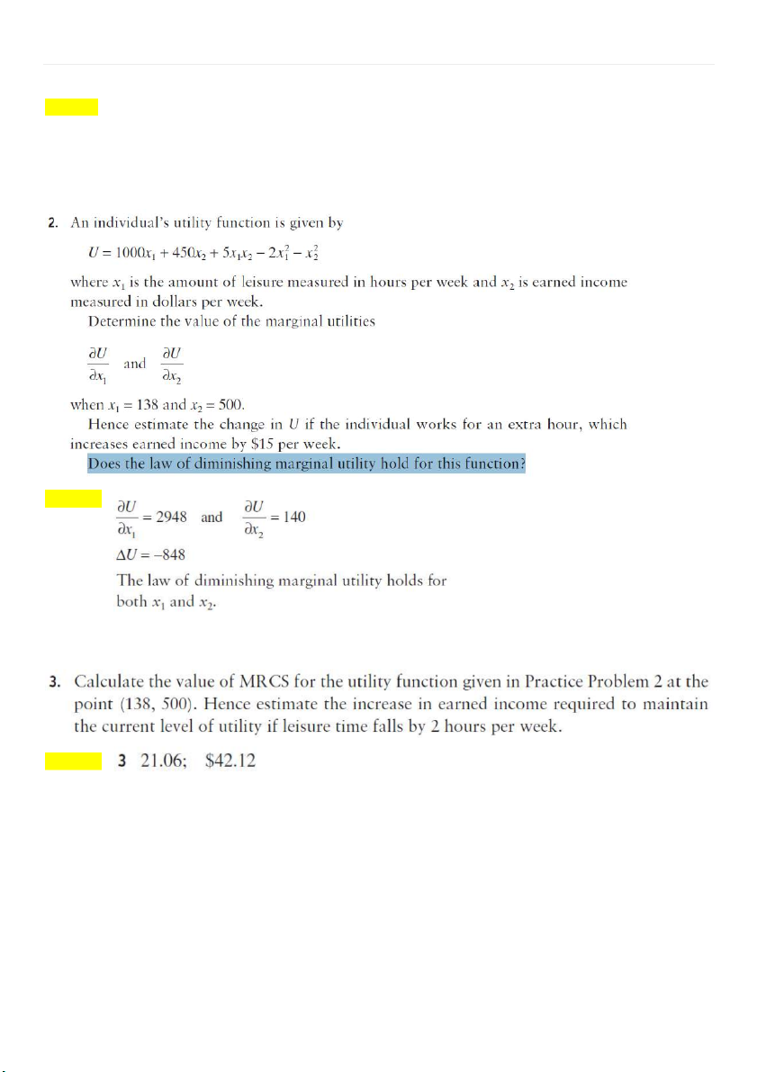
Law of diminishing marginal utility:
+ The consumption of good G1 increases, each additional item of G1 bought confers less
utility than the previous item
+ Does the law of diminishing marginal utility hold for this function?
 The partial derivative of marginal utility ∂U /∂xi (the 2nd order partial derivatives) is negative
3. Calculate the marginal rate of commodity substitution along an indifference curve. -
Marginal rate of commodity substitution is the marginal utility of x1 divided by the marginal utility
of x2: (implicit differentiation) -
The increase in x2 required to maintain the current level of utility when x1 decreases by ∆x1 units: ∆x2 = MRCS x ∆x1
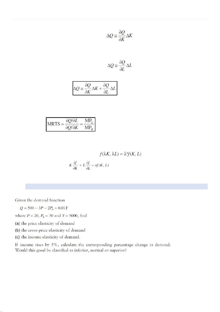
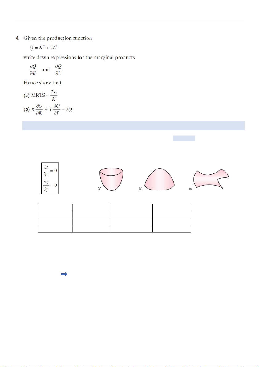
4. Calculate marginal products. Q = f (K, L) -
Marginal product of capital: MPK. If the capital changes by a small amount ΔK, with labor = constant
Contact: ngominhtuyetngoc216@gmail.com
6 | M A T H F O R B U S I N E S S C H A P T E R 5 -
Marginal product of capital: MPL. If the labor changes by a small amount ΔL, with capital = constant -
If K and L both change simultaneously, then the net change in Q can be found from the small increments formula: (isoquant)
5. Calculate the marginal rate of technical substitution along an isoquant.
Marginal rate of technical substitution is the marginal product of labor divided by the marginal product of capital
6. State Euler’s theorem for homogeneous production functions. -
Production function is described as being homogeneous of degree n if, for any number λ - Euler’s theo - rem: EXERCISE (5.2)
1. Calculate partial elasticities.
Contact: ngominhtuyetngoc216@gmail.com
7 | M A T H F O R B U S I N E S S C H A P T E R 5
Solution: a) 20.14 (b) 20.14 (c) 0.12
Percentage change in demand = 5% x 0,12 = 0,006  Normal
2. Calculate marginal utilities. Solution:
3. Calculate the marginal rate of commodity substitution along an indifference curve. Solution:
4. Calculate marginal products and MRTS
Contact: ngominhtuyetngoc216@gmail.com
8 | M A T H F O R B U S I N E S S C H A P T E R 5 III.
Unconstrained optimisation
1. Find and classify stationary points of functions of 2 variables z = f (x, y) (ex: �㔋 = TR – TC) - Find the stationary points:
Solve the simultaneous equations -
Classify stationary points: (*) fxx fyy – (fxy)2 fxx and fyy Figure Minimum > 0 > 0 a Maximum > 0 < 0 b Saddle points < 0 c
2. Tìm giá trị của inputs để output max hoặc min -
Viết ph±ơng trình cÿa output bằng các inputs
Ex: �㔋 = 1000Q1 + 800Q2 – 2Q12 – 2Q1Q2 – Q22 (Output là �㔋, inputs là Q1 và Q2) -
Tìm các partial derivatives cÿa t¿t c¿ các inputs At the stationary point: FQ1 = 0 Q1 =&. FQ2 = 0 Q2 =& -
Thế các giá trị Q1 và Q2 vào b c
¿ng (*) để hÿng minh đó là điểm cÿc đ¿i hoặc cÿc tiểu: By the way, we have &.
Confirming that the output is maximized/minimized at inputs (ex: by producing Q1 and Q2)
Contact: ngominhtuyetngoc216@gmail.com
9 | M A T H F O R B U S I N E S S C H A P T E R 5
3. Find the maximum profit of a firm that sells a single good in different markets with price discrimination. -
Problem: Firm s¿n xu¿t mßt l±ÿng Q hàng hóa vßi TC = & Bán ra 2 thị tr±ßng khác nhau vßi số
l±ÿng và giá hàng hóa ß tÿng thị tr±ßng l¿n l±ÿt là Q1, Q2 và P1, P2
→ Lúc này ta có 1 ptr TC và 2 ptr TR1; TR2 ÿng vßi tÿng thị tr±ßng → �㔋 = (TR1+TR2) – TC - Solution:
+ CHAP 4 (1 variable): Dùng hệ qu¿ �㔋 → MR = MC
+ CHAP 5 (2 variables): Vi¿t ptr �㔋 theo c¿ 2 bi¿n: Q1 và Q2
→ Áp dÿng ph±¡ng pháp ß mÿc 2 đß gi¿i EXERCISE (5.4)
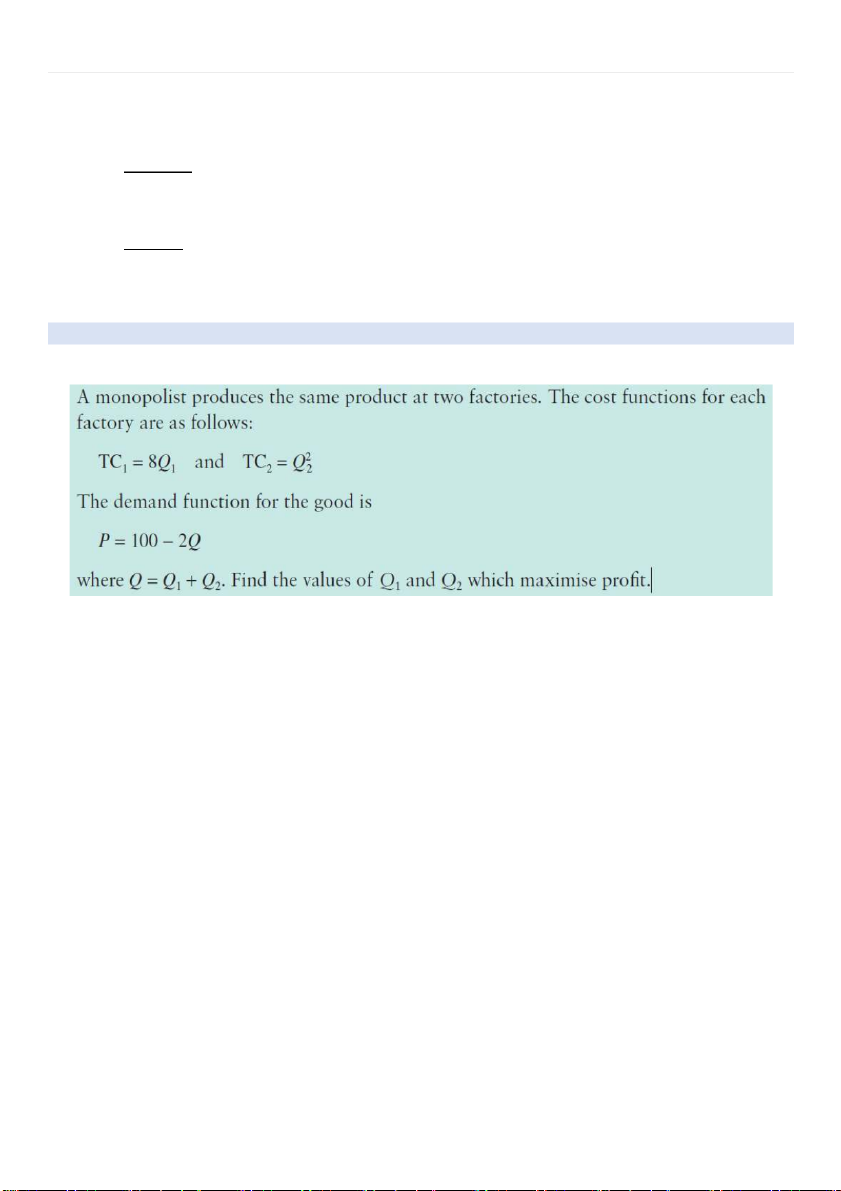
1. Tìm Q1, Q2 để �㕅 max, tính gtr �㕅 max
- The firm’s revenue:
TR = PQ = (100 – 2Q)Q = 100Q 2Q – 2 = 100Q1 + 100Q2 – 2Q12 2Q – 22 4Q – 1Q2(because Q = Q1 + Q2) -
The total cost functions of the firm in both factories: TC = TC1 + TC2 = 8Q1 + Q22 - The firm’s profit:
Π = TR – TC = 100Q1 + 100Q2 – 2Q12 2Q – 22 4Q – 1Q2 – 8Q1 - Q22 = 92Q1 + 100Q2 2Q – 12 – 3Q22 4Q – 1Q2 - At the stationary point:
dΠ / dQ1 = 92 – 4Q1 – 4Q2
dΠ / dQ2 = 100 – 6Q2 – 4Q1  Q1 = 19 & Q2 = 4 -
The second order partial derivatives are 4 ; – 6 and – 4 r – espectively
 Satisfying the condition & fxxfyy (f
– xy)2 = 8 > 0 and fxx < 0; fyy < 0
Confirming that the stationary point is the maximum
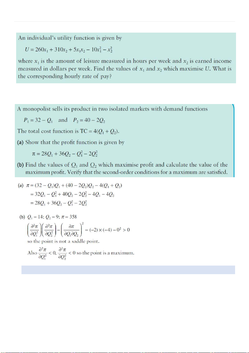
Hence, firm maximises profit at Q1 = 19 and Q2 = 4. 2. Utility
Contact: ngominhtuyetngoc216@gmail.com
10 | M A T H F O R B U S I N E S S C H A P T E R 5
Answer: x1 = 138, x2 = 500; $16.67 per hour.
3. Price discrimination IV.
Constrained optimization
Ph±ơng trình 2 variables nh± III. Unconstrained optimization nh±ng giÿa hai ẩn có m i liên h ố ệ (constrained)
1. Some ratio relates to the constrains.
Contact: ngominhtuyetngoc216@gmail.com
11 | M A T H F O R B U S I N E S S C H A P T E R 5 1.1.
The firm maximises output subject to a cost constraint. -
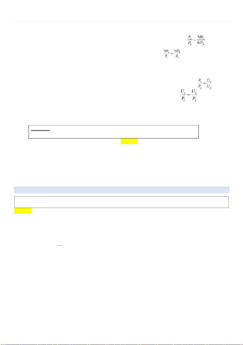
The ratio of the input prices is equal to the ratio of their marginal products: -
The ratio of marginal product to price is the same for all inputs: (both equal to MRTS) 1.2.
The consumer maximises utility subject to a budgetary constraint. -
The ratio of the prices of the goods is equal to the ratio of their marginal utilities: -
The ratio of marginal utility to price is the same for all goods consumed: (both equal to MRCS)
2. Use the method of substitution to solve constrained optimisation problems in economics.
Problem: Use the method of substitution for optimizing
z = f(x, y) subject to φ ( x , y ) = M Solution -
Step 1: Use the constraint φ to expres (x, y) = M s y in terms of x.
(Dựa vào mối liên hệ cÿa x, y đß đ±a ptr z vß 1 variable) -
Step 2: Substitute this expression for y into the objective function z = f (x, y) to write z as a function of x only. -
Step 3: Use the theory of stationary points of functions of one variable to optimise z. (Gi¿i bằng pp cÿa chap 4) EXERCISE (5.5)
1. Find the maximum value of the objective function z = 2x2 2 3xy + 2y + 10
subject to the constraint y = x. Solution: -
Substituting y=x into the objective function z = 2x2 2 3xy + 2y + 10 z = 2x2 2 3x(x) + 2(x) + 10  Z = -x2 + 2x + 10 - At the stationary point:
�㕑�㕧 = -2x + 2 = 0  x = 1 �㕑�㕥  y = x = 1 -
The second – order derivative is (d2z) / (dx2) = -2 < 0 confirming that the stationary point is a maximum. - Hence, z = 2(1)2 3(1 – )(1) + 2(1) + 10 = 11
The maximum value of the objective function z = 2x2 2 3xy + 2y + 10 subject to the constraint y = x is 12
Contact: ngominhtuyetngoc216@gmail.com
12 | M A T H F O R B U S I N E S S C H A P T E R 5
2. A firm’s unit capital and labour costs are $1 and $2 respectively. If the production function is given by Q = 4 LK + L2
find the maximum output and the levels of K and L at which it is achieved when the total input costs are
fixed at $105. Verify that the ratio of marginal product to price is the same for both inputs at the optimum. Solution:
• Find the maximum output: -
The firm’s total cost when it use K units of capital and L units of labour:
TC = K + 2L (A firm’s unit capital and labour costs are $1 and $2 respectively)
By the way, the total input costs are fixed at $105  TC = K + 2L = 105  K = 105 – 2L -
Substituting K = 105 2L into the production function, we have – : Q = 4LK + L2 = 4L(105 2L) + L – 2 = - 7L2 + 420L - At the stationary point:
�㕑�㕄 = - 14L + 420  L = 30 �㕑�㔿
 K = 105 – 2L = 105 – 2(30) = 45 -
The second – order derivative is (d2Q) / (dL2) = - 14 < 0 confirming that the stationary point is a maximum. -
Hence, Q = 4(30)(45) + (30)2 = 6300
The maximum output is 6300 at the levels of capital and labour are 45 and 30 respectively.
• Verify that the ratio of marginal product to price is the same for both inputs at the optimum. -
MPL = �㔕�㕄 = 4K + 2L = 4(45) + 2(30) = 240 �㔕�㔿 V. Lagrange multipliers
1. Use the method of Lagrange multipliers to solve constrained optimisation problems.
Problem: To optimise an objective function f(x, y) subject to a constraint φ ( x , y ) = M
(use method of Lagrange multipliers) Solution: - Step 1
Define a new function (Lagrangian function)
g (x, y, λ) = f (x, y) + λ [ M 2 φ (x, y)] λ: lagrange multipliers - Step 2
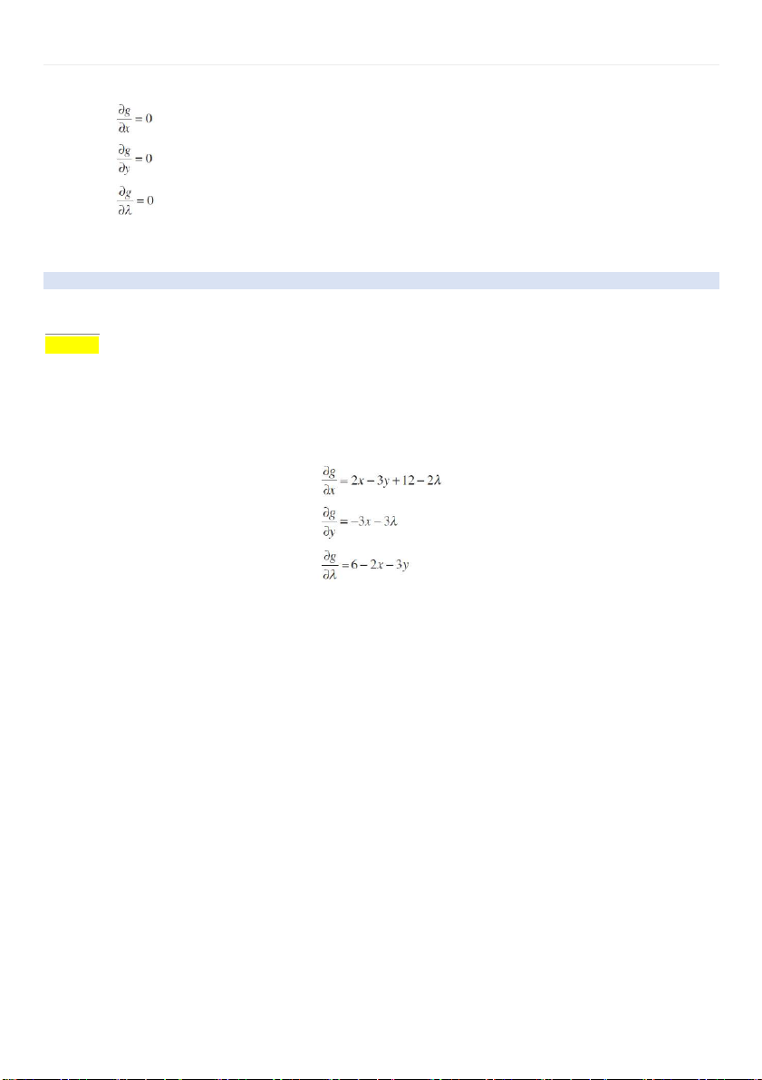
Solve the simultaneous equations:
Contact: ngominhtuyetngoc216@gmail.com
13 | M A T H F O R B U S I N E S S C H A P T E R 5
2. Give an economic interpretation of Lagrange multipliers: the value of λ gives the approximate
change in the optimal value of f due to a 1 unit increase in M. EXERCISE (5.6)
Use the method of Lagrange multipliers to solve constrained optimisation problems.
Problem: Optimise the value of x2 2 3xy + 12x subject to the constraint 2x + 3y = 6 Solution:
• Find out the lagrangian function: - f (x, y) = x2 2 3xy + 12x - φ( x , y ) = 2 x + 3 y - M = 6
 the Lagrangian function is given by g(x, y, λ) = x2 2 3xy + 12x + λ(6 2 2x 2 3y)
• Calculate the three unknowns x, y and λ:
 The values of x, y and λ are -1; 8/3 and 1 respectively.
Hence, substituting x, y, λ into the given function, we deduce the max value of it:
(-1)2 – 3(-1)(8/3) + 12(-1) = -3
Contact: ngominhtuyetngoc216@gmail.com