Choice under Uncertainty - Môn Kinh tế vĩ mô - Đại Học Kinh Tế - Đại học Đà Nẵng

lOMoARcPSD| 49922156
Chapter 5 Choice under Uncertainty Topics to be discussed 1. Describing Risk 2. Preferences Toward Risk 3. Reducing Risk
4. The demand for risky assets
Choice with certainty is reasonably straightforward.
How do we choose when certain variables such as income and prices are uncertain (i.e. making choices with risk)? 5.1 Describing Risk
To measure risk we must know:
o All of the possible outcomes.
o The likelihood that each outcome will occur (its probability).
Interpreting Probability o The likelihood that a given
outcome will occur o Objective Interpretation
Based on the observed frequency of past events o Subjective
Based on perception or experience with or without an observed frequency
Different information or different abilities to process the same information
can influence the subjective probability o Expected Value
The weighted average of the payoffs or values resulting from all possible outcomes.
The probabilities of each outcome are used as weights
Expected value measures the central tendency; the payoff or value expected on average o An Example
Investment in offshore drilling exploration: Two outcomes are possible
• Success -- the stock price increase from $30 to $40/share
• Failure -- the stock price falls from $30 to $20/share Objective Probability
• 100 explorations, 25 successes and 75 failures
• Probability (Pr) of success = 1/4 and the probability of failure = 3/4
Expected Value (EV)Expected Value (EV) An Example: lOMoARcPSD| 49922156
EV Pr(success)($40/share) Pr(failure)($20/share) EV 1 4($40/share ) 3 4($20/share ) EV $25/share Given:
o Two possible outcomes having payoffs X1 and X2 o
Probabilities of each outcome is given by Pr1 & Pr2
Generally, expected value is written as:
E(X) Pr X 1 1 Pr X2 2 ...Pr Xn n Variability
The extent to which possible outcomes of an uncertain even may differ A Scenario
Suppose you are choosing between two part-time sales jobs that have the same expected income ($1,500)
The first job is based entirely on commission.
The second is a salaried position
There are two equally likely outcomes in the first job--$2,000 for a good sales job and
$1,000 for a modestly successful one.
The second pays $1,510 most of the time (.99 probability), but you will earn $510 if
the company goes out of business (.01 probability). Income from Sales Jobs Outcome 1 Outcome 2 Expected
Probability Income ($) ProbabilityIncome ($) Income Job 1: Commission .5 2000 .5 1000 1500 Job 2: Fixed salary .99 1510 .01 510 1500 Income from Sales Jobs Job 1 Expected Income
E(X )1 .5($2000) .5($1000) $ 1500 Job 2 Expected Income lOMoARcPSD| 49922156 E(X ) .99($1510) .01($510)2 $1500
While the expected values are the same, the variability is not.
Greater variability from expected values signals greater risk. Deviation
o Difference between expected payoff and actual payoff
Deviations from Expected Income ($) Outcome 1 Deviation Outcome 2 Deviation Job 1 $2,000 $500 $1,000 -$500 Job 2 1,510 10 510 -900
Variability o Adjusting for negative numbers
o The standard deviation measures the square root of the average of the squares of
the deviations of the payoffs associated with each outcome from their expected value.
The standard deviation is written: Pr 1 X E X1 ( )2 Pr2 X E X2 ( )2
Calculating Variance ($) Deviation Deviation Deviation Standard Outcome 1 Squared Outcome 2 Squared Squared Deviation Job 1 $2,000 $250,000 $1,000
$250,000 $250,000 $500.00 Job 2 1,510 100 510 980,100 9,900 99.50
The standard deviations of the two jobs are: 1 .5($250,000) .5($250,000 1 $250,000 1 500 *Greater Risk lOMoARcPSD| 49922156 2 .99($100) .01($980,100) 2 $9,900 2 99.50
The standard deviation can be used when there are many outcomes instead of only two.
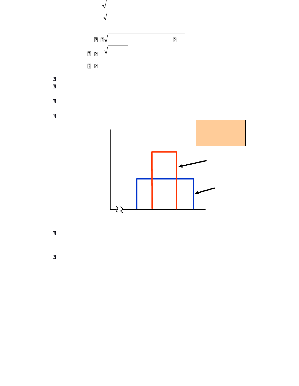
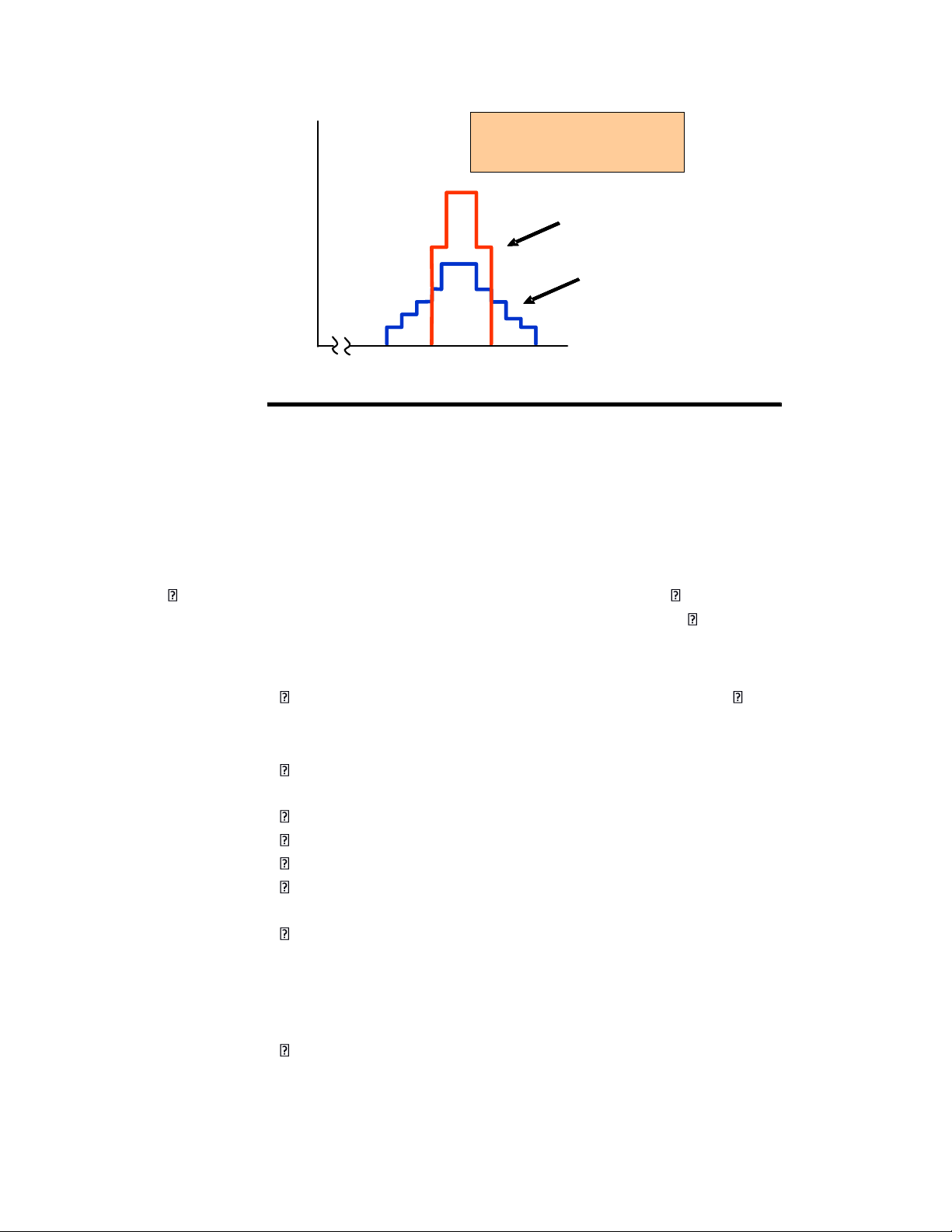
Job 1 is a job in which the income ranges from $1000 to $2000 in increments of $100 that are all equally likely.
Job 2 is a job in which the income ranges from $1300 to $1700 in increments of $100 that, also, are all equally likely. Job 1 has greater spread: greater Probability standard deviation and greater risk than Job 2. 0.2 Job2 0.1 Job 1 Income $1000 $1500 $2000
Outcome Probabilities of Two Jobs (unequal probability of outcomes) o
Job 1: greater spread & standard deviation
o Peaked distribution: extreme payoffs are less likely Decision Making
o A risk avoider would choose Job 2: same expected income as Job 1 with less risk.
o Suppose we add $100 to each payoff in Job 1 which makes the expected payoff = $1600. lOMoARcPSD| 49922156
The distribution of payoffs Probability Job 2
associated with Job 1 has a
greater spread and standard
deviation than those with Job 2. 0.2 Job 1 Income 0.1 $1000 $1500 $2000 Deviation Deviation Expected Standard Outcome 1 Squared
Outcome 2 SquaredIncome Deviation Job 1 $2,100 $250,000 $1,100 $250,000 $1,600 $500 Job 2 1510 100 510 980,100 1,500 99.50
Recall: The standard deviation is the square
root of the deviation squared.
Job 1: expected income $1,600 and a standard deviation of $500.
Job 2: expected income of $1,500 and a standard deviation of $99.50
Which job? o Greater value or less risk? o Example
Suppose a city wants to deter people from double parking. The alternatives …... o Assumptions:
Double-parking saves a person $5 in terms of time spent searching for a parking space. The driver is risk neutral.
Cost of apprehension is zero.
A fine of $5.01 would deter the driver from double parking.
Benefit of double parking ($5) is less than the cost ($5.01) equals a net benefit that is less than 0.
Increasing the fine can reduce enforcement cost:
• A $50 fine with a .1 probability of being caught results in an expected penalty of $5.
• A $500 fine with a .01 probability of being caught results in an expected penalty of $5.
The more risk adverse drivers are, the lower the fine needs to be in order to be effective. lOMoARcPSD| 49922156 5.2 Preferences Toward Risk
Choosing Among Risky Alternatives o Assume
Consumption of a single commodity
The consumer knows all probabilities
Payoffs measured in terms of utility Utility function given Example
o A person is earning $15,000 and receiving 13 units of utility from the job.
o She is considering a new, but risky job.
o She has a .50 chance of increasing her income to $30,000 and a .50 chance of
decreasing her income to $10,000.
o She will evaluate the position by calculating the expected value (utility) of the resulting income.
o The expected utility of the new position is the sum of the utilities associated with
all her possible incomes weighted by the probability that each income will occur.
o The expected utility can be written:
E(u) = (1/2)u($10,000) + (1/2)u($30,000) = 0.5(10) + 0.5(18) = 14
E(u) of new job is 14 which is greater than the current utility of 13 and therefore preferred.
Different Preferences Toward Risk
o People can be risk adverse, risk neutral, or risk loving.
o Risk Averse: A person who prefers a certain given income to a risky income with the same expected value.
o A person is considered risk averse if they have a diminishing marginal utility of income
The use of insurance demonstrates risk aversive behavior. Risk averse o A Scenario
A person can have a $20,000 job with 100% probability and receive a utility level of 16.
The person could have a job with a .5 chance of earning $30,000 and a .5 chance of earning $10,000.
Expected Income = (0.5)($30,000) + (0.5)($10,000) = $20,000
Expected income from both jobs is the same -- risk averse may choose current job
The expected utility from the new job is found:
• E(u) = (1/2)u ($10,000) + (1/2)u($30,000) lOMoARcPSD| 49922156
• E(u) = (0.5)(10) + (0.5)(18) = 14 o E(u) of Job 1 is 16 which is
greater than the E(u) of Job 2 which is 14.
This individual would keep their present job since it provides them with
more utility than the risky job.
They are said to be risk averse. The consumer is risk averse because she would prefer a certain income of $20,000 to a gamble with a .5 probability of $10,000
and a .5 probability of $30,000. 0 10 1516 20 30 Income ($1,000)
A person is said to be risk neutral if they show no preference between a certain income, and
an uncertain one with the same expected value. Risk Loving lOMoARcPSD| 49922156
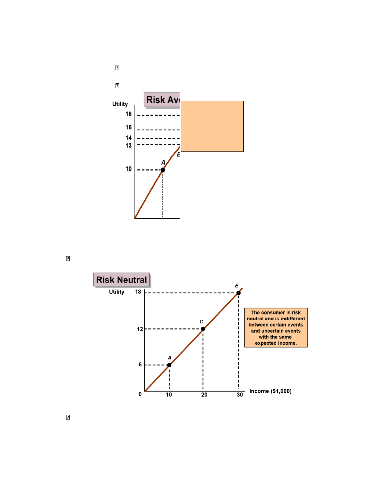
o A person is said to be risk loving if they show a preference toward an uncertain
income over a certain income with the same expected value. Examples:
Gambling, some criminal activity o Risk premium
o The risk premium is the amount of money that a risk-averse person would pay to avoid taking a risk. o A Scenario
o The person has a .5 probability of earning $30,000 and a .5 probability of earning
$10,000 (expected income = $20,000).
o The expected utility of these two outcomes can be found: E(u) = .5(18) + .5(10) = 14 o Question
How much would the person pay to avoid risk? lOMoARcPSD| 49922156
Risk Aversion and Income o Variability in potential payoffs
increases the risk premium. o Example:
A job has a .5 probability of paying $40,000 (utility of 20) and a .5 chance of paying 0 (utility of 0).
The expected income is still $20,000, but the expected utility falls to 10.
Expected utility = .5u($) + .5u($40,000) = 0 + .5(20) = 10
The certain income of $20,000 has a utility of 16.
If the person is required to take the new position, their utility will fall by 6.
The risk premium is $10,000 (i.e. they would be willing to give up $10,000
of the $20,000 and have the same E(u) as the risky job.
o Therefore, it can be said that the greater the variability, the greater the risk premium.
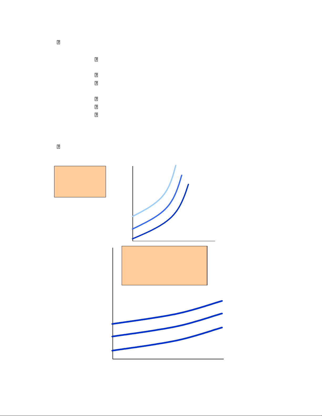
Risk aversion and indifference curves o Combinations of expected income & standard
deviation of income that yield the same utility U3 Highly Risk Averse:An Expected increase in standard Income
U 2 deviation requires a large increase in
U 1 income to maintain satisfaction.
Standard Deviation of Income Expected Slightly Risk Averse: Income
A large increase in standard
deviation requires only a
small increase in income
to maintain satisfaction.
U 3
U 2
U 1
Standard Deviation of Income lOMoARcPSD| 49922156 Example
o Study of 464 executives found that: 20% were risk neutral 40% were risk takers 20% were risk adverse
20% did not respond o Those who liked risky situations did so
when losses were involved. o When risks involved gains the same, executives
opted for less risky situations.
o The executives made substantial efforts to reduce or eliminate risk by delaying
decisions and collecting more information. o 5.3 Reducing Risk
Three ways consumers attempt to reduce risk are: o Diversification o Insurance o Obtaining more information
Diversification o Suppose a firm has a choice of selling air conditioners,
heaters, or both. o The probability of it being hot or cold is 0.5.
o The firm would probably be better off by diversification.
Hot Weather Cold Weather Air conditioner sales $30,000 $12,000 Heater sales 12,000 30,000
* 0.5 probability of hot or cold weather
o If the firms sell only heaters or air conditioners their income will be either $12,000 or $30,000.
o Their expected income would be:
1/2($12,000) + 1/2($30,000) = $21,000 o If the firm divides their time
evenly between appliances their air conditioning and heating sales would be half their original values.
o If it were hot, their expected income would be $15,000 from air conditioners and
$6,000 from heaters, or $21,000.
o If it were cold, their expected income would be $6,000 from air conditioners and
$15,000 from heaters, or $21,000.
o With diversification, expected income is $21,000 with no risk.
o Firms can reduce risk by diversifying among a variety of activities that are not closely related. The Stock market o Discussion Questions
How can diversification reduce the risk of investing in the stock market? lOMoARcPSD| 49922156
Can diversification eliminate the risk of investing in the stock market? Insurance
o Risk averse is willing to pay to avoid risk.
o If the cost of insurance equals the expected loss, risk averse people will buy enough
insurance to recover fully from a potential financial loss. Insurance Burglary No Burglary Expected Standard (Pr = .1)
(Pr = .9) Wealth Deviation No $40,000 $50,000 $49,000 $9,055 Yes 49,000 49,000 49,000 0
o While the expected wealth is the same, the expected utility with insurance is greater
because the marginal utility in the event of the loss is greater than if no loss occurs.
o Purchases of insurance transfer wealth and increases expected utility. o The law of large Numbers
Although single events are random and largely unpredictable, the average
outcome of many similar events can be predicted. Examples
• A single coin toss vs. large number of coins
• Whom will have a car wreck vs. the number of wrecks for a large group of drivers o Actuarial Fairness Assume:
• 10% chance of a $10,000 loss from a home burglary
• Expected loss = .10 x $10,000 = $1,000 with a high risk (10% chance of a $10,000 loss)
• 100 people face the same risk lOMoARcPSD| 49922156 Then:
• $1,000 premium generates a $100,000 fund to cover losses • Actual Fairness
• When the insurance premium = expected payout o Example A Scenario:
• Price of a house is $200,000
• 5% chance that the seller does not own the house
Risk neutral buyer would pay: (.95[200,000] .05[0] 190,000
Risk averse buyer would pay much less
By reducing risk, title insurance increases the value of the house by an
amount far greater than the premium.
Value of Complete Information o The difference between the expected value of a choice
with complete information and the expected value when information is incomplete.
o Suppose a store manager must determine how many fall suits to order: 100 suits cost $180/suit 50 suits cost $200/suit
The price of the suits is $300
Unsold suits can be returned for half cost.
The probability of selling each quantity is .50. Expected Sale of 50 Sale of 100 Profit 1. Buy 50 suits $5,000 $5,000 $5,000 2. Buy 100 suits 1,500 12,000 6,750 With incomplete information:
o Risk Neutral: Buy 100 suits o Risk Averse: Buy 50 suits
The expected value with complete information is $8,500.
o 8,500 = .5(5,000) + .5(12,000)
The expected value with uncertainty (buy 100 suits) is $6,750.
The value of complete information is $1,750, or the difference between the two (the
amount the store owner would be willing to pay for a marketing study).
5.4 The demand for risky assets Assets
o Something that provides a flow of money or services to its owner. lOMoARcPSD| 49922156
The flow of money or services can be explicit (dividends) or implicit (capital gain). Capital Gain
o An increase in the value of an asset, while a decrease is a capital loss. Risky and Risk less Assets o Risky Asset
Provides an uncertain flow of money or services to its owner. Examples
apartment rent, capital gains, corporate bonds, stock prices o Risk less Asset
Provides a flow of money or services that is known with certainty. Examples
short-term government bonds, short-term certificates of deposit Asset Returns o Return on an Asset
The total monetary flow of an asset as a fraction of its price. o Real Return of an Asset
The simple (or nominal) return less the rate of inflation. Asset Returns Monetary Flow Asset Return Purchase Price Flow $100/yr. Asset Return 10 % Bond Price $1,000
Expected versus actual returns o Expected Return
Return that an asset should earn on average o Actual Return Return that an asset earns o Risk Real Rate of (standard lOMoARcPSD| 49922156 Return (%) deviation,%)
Common stocks (S&P 500) 9.5 20.2
Long-term corporate bonds 2.7 8.3 U.S. Treasury bills 0.6 3.2 o
Higher returns are associated with greater risk. o
The risk-averse investor must balance risk relative to return
The trade-off between risk and return o An investor is
choosing between T-Bills and stocks:
T-bills (riskless) versus Stocks (risky)
Rf = the return on risk free T-bills
Expected return equals actual return when there is no risk o
An investor is choosing between T-Bills and stocks:
Rm = the expected return on stocks
rm = the actual returns on stock o At the time of the investment
decision, we know the set of possible outcomes and the likelihood of each, but
we do not know what particular outcome will occur. o
The risky asset will have a higher expected return than the risk free asset (Rm
> Rf). o Otherwise, risk-averse investors would buy only T-bills. o How to allocate savings:
b = fraction of savings in the stock market
1 – b = fraction in T-bills
Investment PortfolioExpected Return:
Rp: weighted average of the expected return on the two assets
Rp = bRm + (1-b)Rf
If Rm = 12%, Rf = 4%, and b = 1/2
Rp = 1/2(.12) + 1/2(.04) = 8% o Question How risky is their portfolio? o
Risk (standard deviation) of the portfolio
is the fraction of the portfolio invested in the risky
asset times the standard deviation of that asset: b p m lOMoARcPSD| 49922156
The Investor’s Choice ProblemThe Investor’s Choice Problem Determining b: b R) R bR f p m (1 Rp R b R Rf ( m f ) b p / m (R R ) R Rp f m f p m
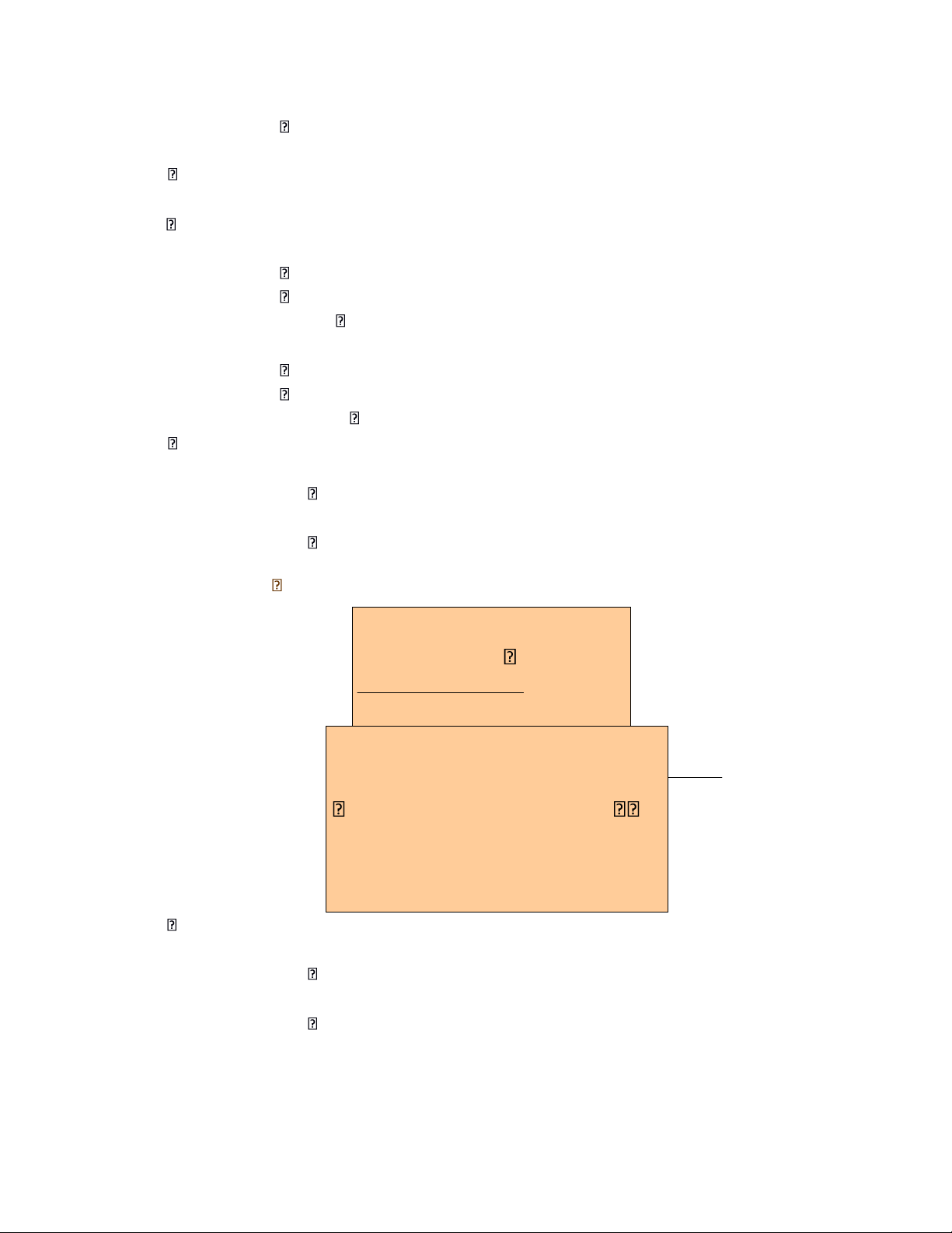
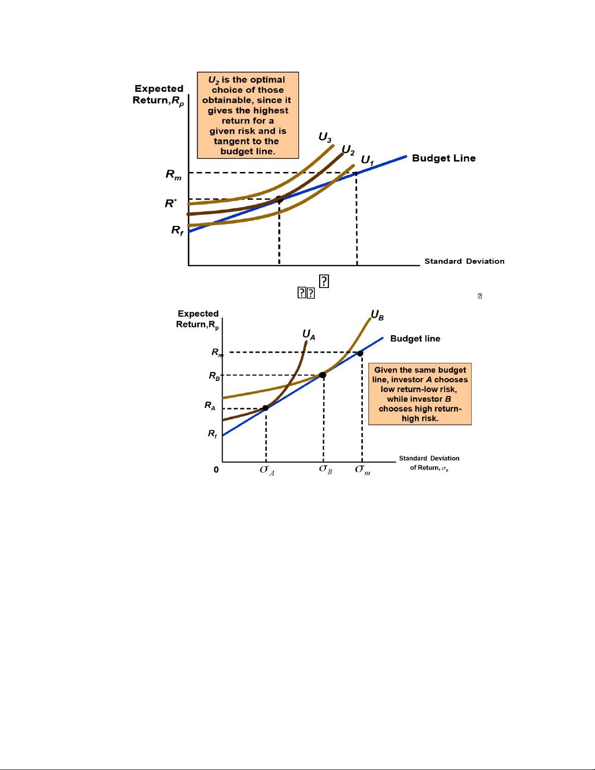
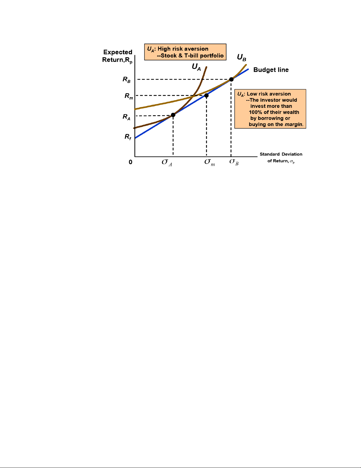
Risk and the Budget LineRisk and the Budget Line Observations
1) The final equation Rp Rf (Rm R )f p m
is a budget line describing the tradeoff
between risk and expected ( p) return .(Rp)
Observations: Rp Rf (Rm R )f p m
2) Is an equation for a straight line: R , R , and m f m are constants
3) Slope (R m R )/f m
• 4) Expected return, RP, increases as risk increases.
• 5) The slope is the price of risk or the risk-return trade-off. lOMoARcPSD| 49922156 0 m of Return, p lOMoARcPSD| 49922156