Chương 6 Giải pháp số cho hệ phương trình tuyến tính | Trường Đại học Kinh tế Quốc dân

NATIONAL ECONOMIC UNIVERSITY
FACULTY OF INFORMATION TECHNOLOGY CHAPTER 6
NUMERICAL SOLUTION OF SYSTEMS OF LINEAR EQUATIONS OBJECTIVES
 Describe methods for solving systems of linear algebraic equations: ➢ Gauss Method ➢ Simple Iteration Method 2 CONTENT 1. Introduction 2.
Existence and uniqueness of solutions to systems of linear equations 3. Gauss Method 4. Simple Iteration Method 3 1. INTRODUCTION
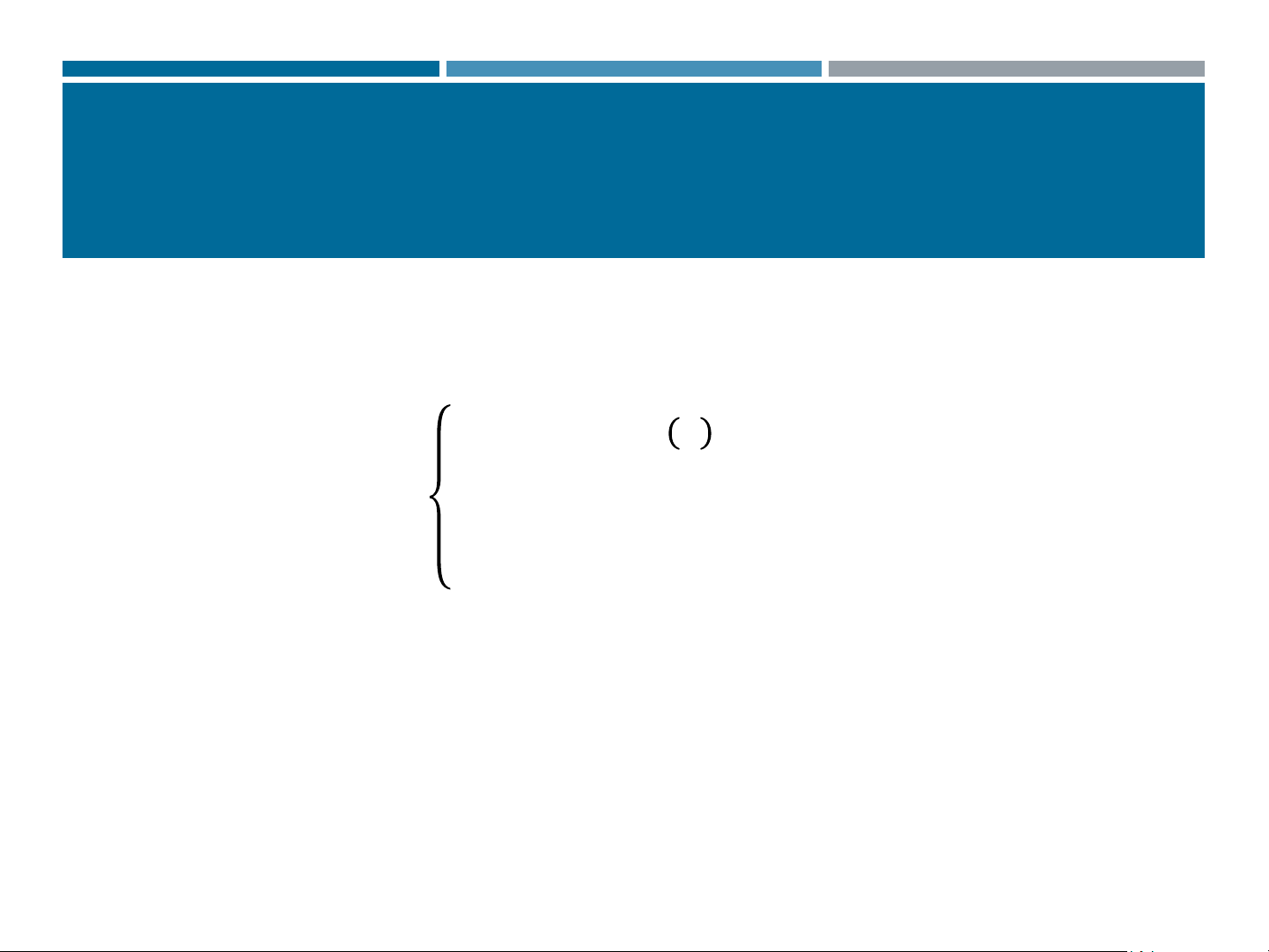
𝑎11𝑥1 + 𝑎12𝑥2 + ⋯ + 𝑎1𝑛𝑥𝑛 = 𝑓1
Consider the system of equations 𝑎 :
21𝑥1 + 𝑎22𝑥2 + ⋯ + 𝑎2𝑛𝑥𝑛 = 𝑓2 (1) … … … … . .
𝑎𝑛1𝑥1 + 𝑎𝑛2𝑥2 + ⋯ + 𝑎𝑛𝑛𝑥𝑛 = 𝑓𝑛 where: •
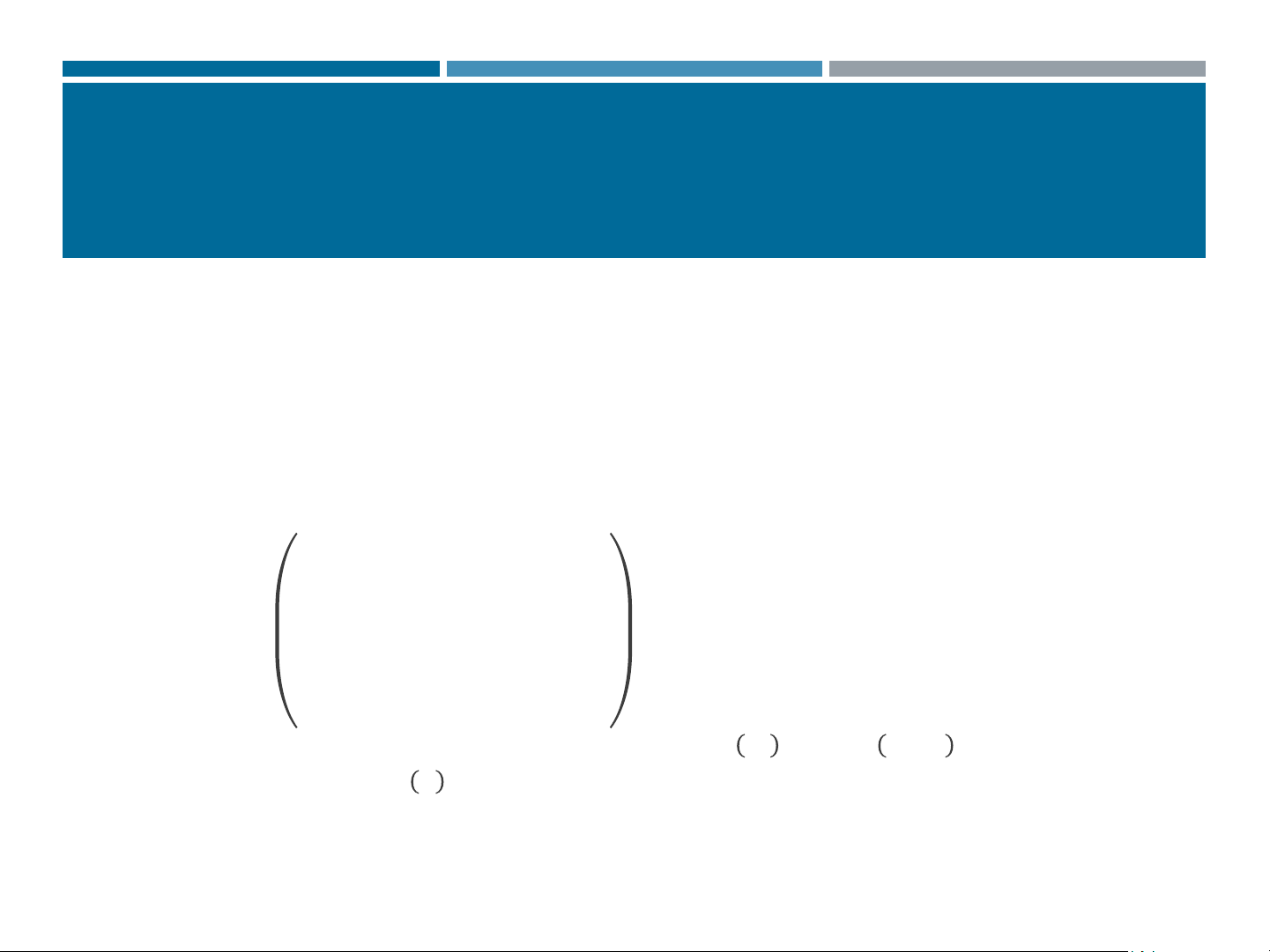
𝑎𝑖𝑗 is the coefficient of the variable 𝑥𝑗 in the 𝑖-th equation. 𝑎11 𝑎12 . . . 𝑎1𝑛 •
𝑓 is the right-hand side of the 𝑖 𝑖-th equation 𝑎21 𝑎22 . . . 𝑎2𝑛 • 𝑥 . . . . . . . .
𝑗 are the unknowns of the system 𝑎 •
The matrix A is called the coefficient matrix. 𝑛1 𝑎𝑛1 . . . 𝑎𝑛𝑛 4 1. INTRODUCTION 𝑓 𝑥1 The vectors: 1 𝑓 𝑥2 𝑓 = 2 𝑥 = . . . . . . 𝑓 𝑥 𝑛 𝑛
Are called the right-hand side vector and the vector of unknowns of system We can denote: 𝑓 = 𝑓 𝑇 1, 𝑓2, … , 𝑓𝑛 𝑥 = 𝑥 𝑇 1, 𝑥2, … , 𝑥𝑛
System (1) can be represented as: 𝐴𝑥 = 𝑓 5
2. EXISTENCE AND UNIQUENESS OF
SOLUTIONS TO SYSTEMS OF LINEAR Cramer’s Theorem
If the determinant ∆ ≠ 0, i.e., if the system is non-singular, then system
(1) has a unique solution given by the formula: ∆ 𝑥 = 𝑖 (2) ∆ Remark:
The result is theoretically elegant, but computing the solution using (2) requires considerable effort.
=> Approximate methods are preferred. 6 3. GAUSS METHOD Idea:
Use successive elimination of the unknowns to transform the given
system into an upper triangular system, then solve the triangular system from bottom to top. Example: 2𝑥 ቊ 1 + 𝑥2 = 1 4𝑥1 + 6𝑥2 = 3
Eliminating 𝑥1 from the second equation, we obtain: 2𝑥 ቊ 1 + 𝑥2 = 1 4𝑥2 = 1
The system is now in triangular form. Solving from bottom to top gives the solution of the system. 7 3. GAUSS METHOD
Consider a three-variable system
𝑎11𝑥1 + 𝑎12𝑥2 + 𝑎13𝑥3 = 𝑎14
ቐ𝑎21𝑥1 + 𝑎22𝑥2 + 𝑎23𝑥3 = 𝑎24 (*)
𝑎31𝑥1 + 𝑎32𝑥2 + 𝑎33𝑥3 = 𝑎34
Transform to an upper triangular form
𝑥1 + 𝑏12𝑥2 + 𝑏13𝑥3 = 𝑏14 ቐ 𝑥2 + 𝑏23𝑥3 = 𝑏 (**) 24 𝑥3 = 𝑏34
The process of reducing (*) to (**) is called forward elimination.
The process of solving (**) is called back substitution 8 3. GAUSS METHOD Forward elimination Step 1: Eliminate x1.
Assume a11≠ 0 . Dividing (1) by a11 we obtain: x (1) (1) (1) 1 + a + a = a (4) 12 13 14
Use (4) to eliminate x1 from equations (2) and (3) by applying
multiplication and addition/subtraction operations a Where: a(1)= 1j 1j a11
Step 2: Similarly, eliminate 𝑥2 Back substitution
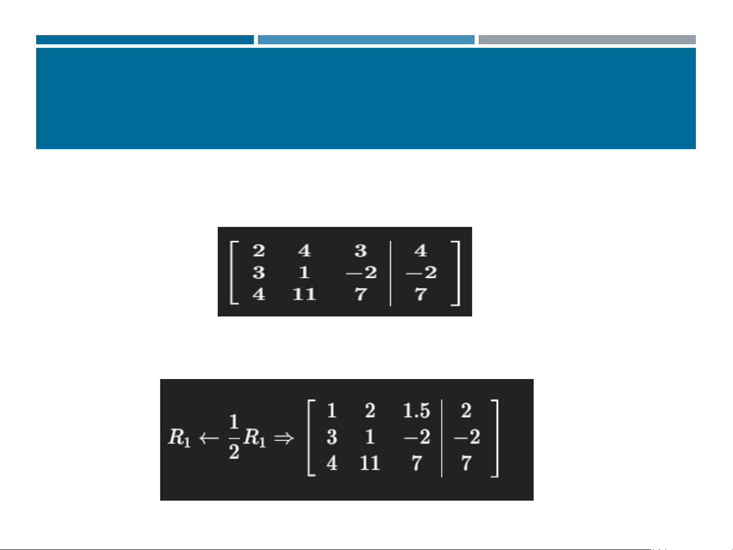
Solve the triangular system to obtain the solution 9 3. GAUSS METHOD Example Solving Linear Systems 2𝑥1+4𝑥2 + 3𝑥3 = 4 1
3𝑥1 + 𝑥2 − 2𝑥3 = −2 (2) 4𝑥1 + 11𝑥2 + 7𝑥3 = 7 (3) 1. Forward elimination. Step 1: Eliminate x1 Step 2 :Eliminate x2 2. Back substitution Solve the triangular system
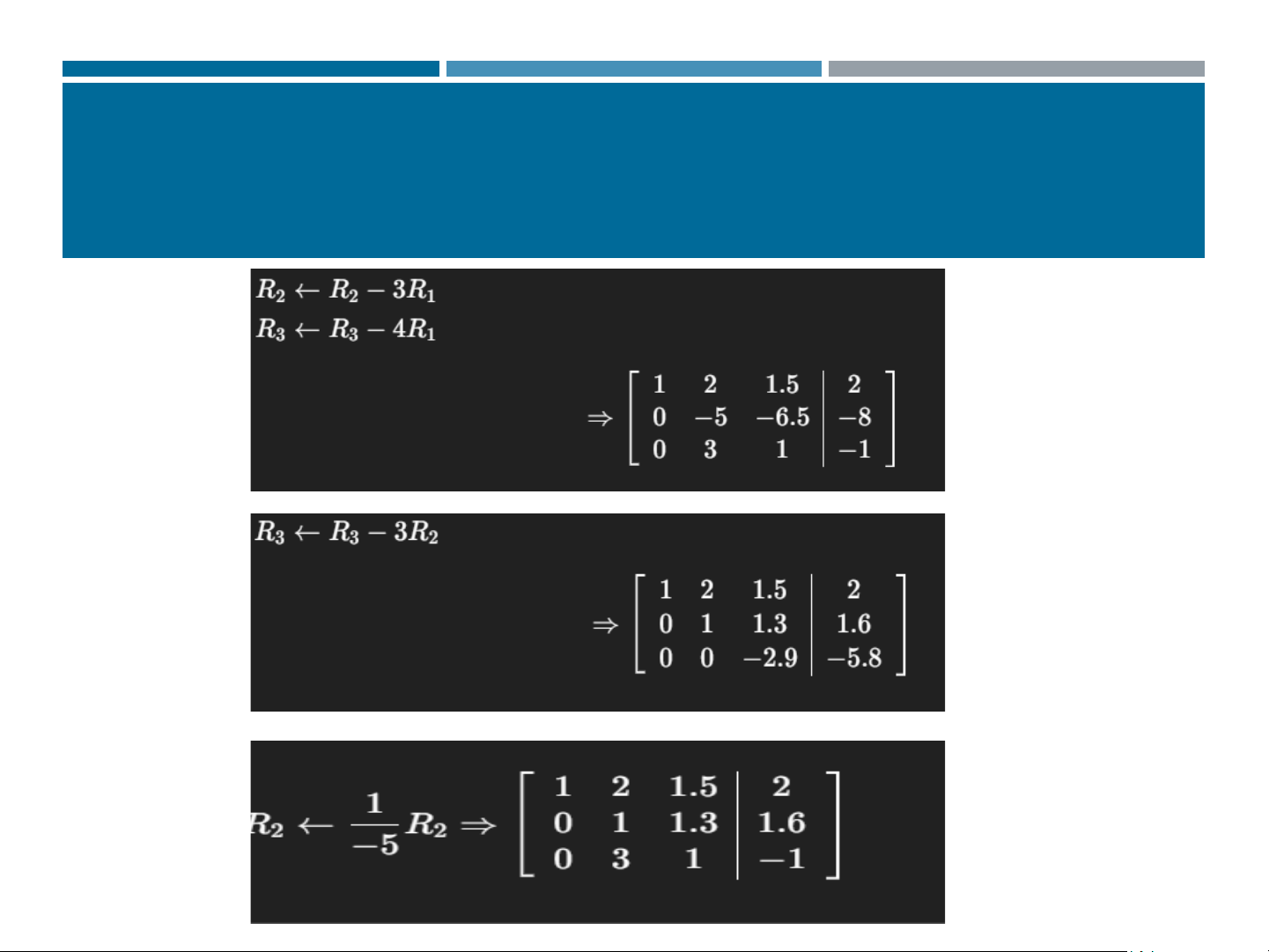
3. Conclude the solution 10 3. GAUSS METHOD 1. Coefficient matrix
2. Transform into upper triangular form 11 3. PHƯƠNG PHÁP GAUSS 12 3. GAUSS METHOD
3. Solving the upper triangular system from bottom to top 𝑥1= 1 1 𝑥2 = −1 (2) 𝑥3 = 2 (3) 13 3. GAUSS METHOD Exercise: Solving Linear Systems 1.
3𝑥 + 2𝑦 − 5𝑧 = −3 (1) 2𝑥 + 𝑦 + 3𝑧 = 11 (2)
4𝑥 + 3𝑦 − 12𝑧 = −15 (3) 2. 5𝑥 + 2𝑦 − 3𝑧 = 9 (1) 2𝑥 + 𝑦 − 4𝑧 = 6 (2) 8𝑥 + 3𝑦 − 5𝑧 = 15 (3) 14 4. SIMPLE INTERATION METHOD a. Description
Consider the Linear Systems Equantions: 𝐴𝑥 = 𝑓 (1)
We seek to transform this system into an equivalent system of the form: 𝑥 = 𝐵𝑥 + 𝑔 (2)
where and are derived from and in some manner. 𝐵 𝑔 𝐴 𝑓 𝒃11 𝒃12 . . . 𝒃1𝑛 Suppose B= 𝒃21 𝒃22 . . . 𝒃2𝑛 . . . . . . . . 𝒃𝑛1 𝒃𝑛1 . . . 𝒃𝑛𝑛
We construct the iteration formula:
𝑥 𝑚 = 𝐵. 𝑥 𝑚−1 + 𝑔 (3)
with an initial vecto 𝑥 𝑜 given
The method based on formula (3) is called the simple iteration method,
and B is referred to as the iteration matrix. 15 4. SIMPLE INTERATION METHOD b. Convergence Definition 1: Suppose α = α 𝑇 1, α2, … , α𝑛
s the solution of the given system (1). If 𝑥 𝑚 → 𝛼 𝑖
𝑖 𝑎𝑠 𝑚 → ∞ , 𝑖 = 1, 2, … , 𝑛 then we say that the iteration method (3) converges. Definition 2: For a vecto 𝑧 = 𝑧 𝑇 1, 𝑧2, … , 𝑧𝑛
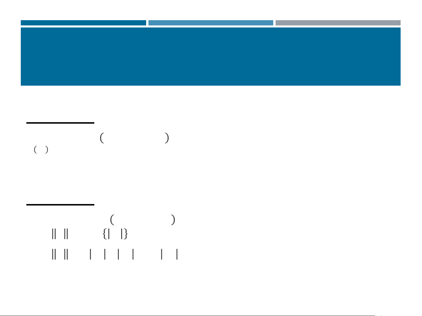
, the following quantities are defined: 𝑧 o=max 𝑧𝑖 𝑧 = 𝑧 1 1 + 𝑧2 + … 𝑧𝑛
which are called norms of the vector 𝑧 16 4. SIMPLE INTERATION METHOD Definition 3:
For a square matrix 𝐵 = 𝑏𝑖𝑗 the matrix norms are defined: 𝐵 𝑛 o=maxi σ𝑗=1 𝑏𝑖𝑗 𝐵 𝑛 1=maxj σ𝑖=1 𝑏𝑖𝑗 Theorem:
If 𝐵 p < 1 (4) then the iterative method converges for any initial
approximation, and the error can be estimated as 𝐵 𝑝 𝑥 𝑚 − 𝛼 p ≤ . 𝑥 𝑚 − 𝑥 𝑚−1 1− 𝐵 𝑝 p (*) 𝐵 𝑝 𝑥 𝑚 − 𝛼 p ≤ . 𝑥 1 − 𝑥 0 1− 𝐵 𝑝 p
Where: p=0 if 𝐵 o<1; p=1 if 𝐵 1<1 17 4. SIMPLE INTERATION METHOD c. Example
Consider the systems of linear equations
4𝑥1 + 0.24𝑥2 − 0.08𝑥3 = 8 (1)
0.09𝑥1 + 3𝑥2 − 0.15𝑥3 = 9 (2)
0.04𝑥1 − 0.08𝑥2 + 4𝑥3 = 20 (3)
Divide each equation by its diagonal coefficient:
𝑥1 = −0.06𝑥2 + 0.02𝑥3 + 2
ቐ𝑥2 = −0.03𝑥1 + 0.05𝑥3 + 3
𝑥3 = −0.01𝑥1 + 0.02𝑥2 + 5
We have: 𝑥 = 𝐵𝑥 + 𝑔 18 4. SIMPLE INTERATION METHOD 0 −0.06 0.02 𝟐 B= −0.03 0 0.05 g= 𝟑 𝟓 −0.01 0.02 0
Check the convergence condition
σ3𝑗=1 𝑏1𝑗 =0+0.06+0.02=0.08
σ3𝑗=1 𝑏2𝑗 =0.03+0+0.05=0.08
σ3𝑗=1 𝑏3𝑗 =0.01+0.02+0=0.03 𝐵 𝑛
o=maxi σ𝑗=1 𝑏𝑖𝑗 =max (0.08, 0.08, 0.03)=0.08 <1 19 4. SIMPLE INTERATION METHOD
According to the theorem: the iterative method converges with the iterative formula 𝑚 𝑥
= 𝐵. 𝑥 𝑚−1 + 𝑔 for any 𝑥 0 choosen
Suppose we take: 𝑥 0 = (0,0,0)T 0 𝑥 0 = 0 0 20