Confidence Intervals for Mean (σ Known): Chapter 8 Summary môn Xác suất thống kê| Đại học Duy Tân

14:27, 11/01/2026
Confidence Intervals for Mean (σ Known): Chapter 8 Summary - Studocu
280 CHAPTER 8 CONFIDENCE INTERVAL ESTIMATION
LEARNING After studying this chapter you should be able to:
OBJECTIVES 1 construct and interpret confidence interval estimates for the mean
2 construct and interpret confidence interval estimates for the proportion
3 determine the sample size necessary to develop a confidence interval for the mean or proportion
4 recognise how to use confidence interval estimates in auditing
Statistical inference is the process of using sample results to draw conclusions about the char-
acteristics of a population. Inferential statistics enables you to estimate unknown population
characteristics such as a population mean or a population proportion. Two types of estimates point estimate
are used to estimate population parameters: point estimates and interval estimates. A point
A single value calculated from a estimate is the value of a single sample statistic. A confidence interval estimate is a range of
sample which is used to estimate numbers, called an interval, constructed around the point estimate. The process used to construct
an unknown population parameter. confidence intervals tells us that the population parameter is located somewhere within the inter-
val in a known percentage of the intervals that could be constructed from different samples. confidence interval estimate
Suppose that you would like to estimate the mean number of hours of paid work under-
A range of numbers constructed about the point estimate.
taken per week during term time by students in your university. The mean hours of paid work
for all the students is an unknown population mean, denoted by μ. You select a sample of
–, is a point estimate of the
students and find that the sample mean is 14.8. The sample mean, X
population mean μ. How accurate is 14.8? To answer this question you must construct a confi- dence interval estimate.
In this chapter you will learn how to construct and interpret confidence interval estimates.
–, is a point estimate of the population mean μ. However, the Recall that the sample mean, X
sample mean will vary from sample to sample because it depends on the items selected in the
sample. By taking into account the known variability from sample to sample (see Section 7.2
on the sampling distribution of the mean), you will learn how to develop the interval estimate
for the population mean. The interval constructed will have a specified confidence of correctly
estimating the value of the population parameter μ. In other words, there is a specified confi-
dence that μ is somewhere in the range of numbers defined by the interval.
Suppose that after studying this chapter you find that a 95% confidence interval for the
mean number of hours students at your university are employed in paid work per week is
(14.75 8 μ 8 14.85). You can interpret this interval estimate by stating that you are 95% con-
fident that the mean number of hours per week of paid work undertaken by students at your
university is between 14.75 and 14.85. However, there is still a possibility that the mean num-
ber of hours is below 14.75 or above 14.85.
After learning about the confidence interval for the mean, we look at how to develop an
interval estimate for the population proportion. Then we consider how large a sample to select
when constructing confidence intervals, and how to perform several important estimation pro- 14:27, 11/01/2026
Confidence Intervals for Mean (σ Known): Chapter 8 Summary - Studocu g , p p p
cedures that accountants use when performing audits.
8.1 CONFIDENCE INTERVAL ESTIMATION FOR THE MEAN (σ KNOWN)
In Section 7.2 we used the Central Limit Theorem and knowledge of the population distribution
to determine the percentage of sample means that fall within certain distances of the population
mean. For instance, in the shampoo-bottling example used throughout Chapter 7, 95% of all
Copyright © Pearson Australia (a division of Pearson Australia Group Pty Ltd) 2019— 9781488617249 — Berenson/Basic Business Statistics 5e 14:27, 11/01/2026
Confidence Intervals for Mean (σ Known): Chapter 8 Summary - Studocu
8.1 CONFIDENCE INTERVAL ESTIMATION FOR THE MEAN (σ KNOWN) 281
sample means are between 494.12 and 505.88 mL. This statement is based on deductive reasoning. Deductive reasoning
However, inductive reasoning is what we need here. Reasoning that starts with a
We need inductive reasoning because, in statistical inference, you use the results of a hypothesis and examines
possibilities to move to a specific
single sample to draw conclusions about the population, not vice versa. Suppose that in the conclusion.
shampoo-bottling example you wish to estimate the unknown population mean using the
information from only a sample. Thus, rather than take μ ± (1.96) (σ⁄∙∙
n) to find the upper Inductive reasoning –, for the Reasoning that uses specific
and lower limits around μ, as in Section 7.2, you substitute the sample mean, X – ± (1.96) (σ⁄∙∙
observations to make a general unknown μ and use X
n) as an interval to estimate the unknown μ. Although in conclusion. –, in order to understand
practice you select a single sample of size and calculate the mean n X
the full meaning of the interval estimate you need to examine a hypothetical set of all possi- ble samples of n values.
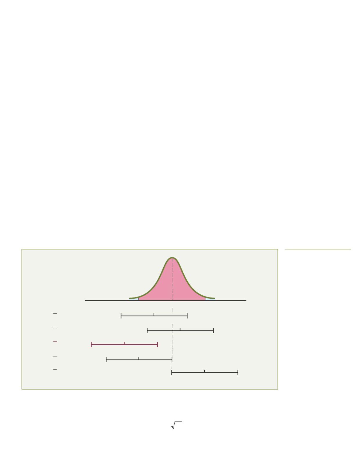
Figure 8.1 shows the actual population distribution of shampoo bottle contents at the top with
a mean value of 500 and five confidence intervals for the population mean based on five different
sample means. Suppose that a sample of n = 25 bottles has a mean of 496.2 mL. The interval devel-
oped to estimate μ is 496.2 ± (1.96)(15)⁄(∙∙ 25) or 496.2 ± 5.88. The interval estimate of μ is: 490.32 8 μ 502.08 8
Because the population mean μ (equal to 500) is included within the interval, this sample has
led to a correct statement about μ (see Figure 8.1). Figure 8.1 Confidence interval estimates for five different samples of n = 25 taken from a population where μ = 500 and σ = 15 494.12 505.88 500 X1 = 496.2 490.32 496.2 502.08 X2 = 501.6 495.72 501.6 507.48 X3 = 493.0 487.12 493.0 498.88 X4 = 494.12 488.24 494.12 500 X5 = 505.88 500 505.88 511.76
To continue this hypothetical example, suppose that for a different sample of n = 25 bottles
the mean is 501.6. The interval developed from this sample is: 501.6 ± (1.96)(15)/( 25)
or 501.6 ± 5.88. The estimate is: 495.72 8 μ 507.48 8 14:27, 11/01/2026
Confidence Intervals for Mean (σ Known): Chapter 8 Summary - Studocu
Because the population mean μ (equal to 500) is also included within this interval, this state- ment about μ is correct.
Now, before you begin to think that correct statements about μ are always made by
developing a confidence interval estimate, suppose a third hypothetical sample of n = 25
bottles is selected and the sample mean is equal to 493 mL. The interval developed here is
493 ± (1.96) (15)⁄(∙∙ 25) or 493 ± 5.88. In this case, the interval estimate of μ is: 487.12 8 μ 498.88 8
Copyright © Pearson Australia (a division of Pearson Australia Group Pty Ltd) 2019— 9781488617249 — Berenson/Basic Business Statistics 5e 14:27, 11/01/2026
Confidence Intervals for Mean (σ Known): Chapter 8 Summary - Studocu
282 CHAPTER 8 CONFIDENCE INTERVAL ESTIMATION
This estimate is not a correct statement, because the population mean μ is not included in the
interval developed from this sample (see Figure 8.1). Thus, for some samples the interval estimate
of μ is correct but for others it is incorrect. In practice, only one sample is selected and, because
the population mean is unknown, you cannot determine whether the interval estimate is correct.
To resolve this dilemma of sometimes having an interval that provides a correct estimate
and sometimes having an interval that provides an incorrect estimate, you need to determine the
proportion of samples producing intervals that result in correct statements about the population – = 494.12 mL
mean μ. To do this, consider two other hypothetical samples: the case in which X
– = 505.88 mL. If X– = 494.12, the interval is 494.12 ± (1.96)(15)⁄(∙∙ and the case in which X 25)
or 494.12 ± 5.88. This leads to the following interval: 488.24 8 μ 500.00 8
Because the population mean of 500 is at the upper limit of the interval, the statement is correct (see Figure 8.1).
– = 505.88, the interval is 505.88 ± (1.96)(15)⁄(∙∙ When X
25) or 505.88 ± 5.88. The interval for the sample mean is: 500.00 8 μ 51 8 1.76
In this case, because the population mean of 500 is included at the lower limit of the interval, the statement is correct.
Figure 8.1 shows that when the sample mean falls anywhere between 494.12 and
505.88 mL, the population mean is included somewhere within the interval. In Section 7.2 we
found that 95% of the sample means fall between 494.12 and 505.88 mL. Therefore, 95% of all
samples of n = 25 bottles have sample means that include the population mean within the inter-
val developed. The interval from 494.12 to 505.88 is referred to as a 95% confidence interval.
Because, in practice, you select only one sample and μ is unknown, you never know for sure
whether the specific interval includes the population mean or not. However, if you take all possible
samples of n and calculate their sample means, 95% of the intervals will include the population
mean and only 5% of them will not. In other words, there is 95% confidence that the population
mean is somewhere in the interval. Thus, we can interpret the confidence interval above as follows:
LEARNING OBJECTIVE 1 I am 95% confident that the mean amount of shampoo in the population of bottles is Construct and interpret
somewhere between 494.12 and 505.88 mL. confidence intervals for the mean
In some situations, you might want a higher degree of confidence (such as 99%) of includ-
ing the population mean within the interval. In other cases, you might accept less confidence
(such as 90%) of correctly estimating the population mean. level of confidence
In general, the level of confidence is symbolised by (1 - α) * 100%, where α is the area in Represents the percentage of
the tails of the distribution that is outside the confidence interval. The area in the upper tail of the distribution is
intervals, based on all samples of a
α/2, and the area in the lower tail of the distribution is α/2. We can use Equa-
certain size, which would contain the population parameter.
tion 8.1 to construct a (1 - α) 100% confidence interv *
al estimate of the mean with σ known.
CONFIDENCE INTERVAL FOR A MEAN (σ KNOWN) 14:27, 11/01/2026
Confidence Intervals for Mean (σ Known): Chapter 8 Summary - Studocu σ X ± Z n or σ σ X − Z ⩽ μ ⩽ X + Z (8.1) n n
where Z = the value corresponding to a cumulative area of 1 - α/2 from the standard-
ised normal distribution – that is, an upper-tail probability of α/2.
Copyright © Pearson Australia (a division of Pearson Australia Group Pty Ltd) 2019— 9781488617249 — Berenson/Basic Business Statistics 5e 14:27, 11/01/2026
Confidence Intervals for Mean (σ Known): Chapter 8 Summary - Studocu
8.1 CONFIDENCE INTERVAL ESTIMATION FOR THE MEAN (σ KNOWN) 283
The value of Z needed for constructing a confidence interval is called the critical value for critical value
the distribution. For a 95% confidence interval the value of α is 0.05. The critical Z value cor-
The value in a distribution that cut
responding to a cumulative area of 0.9750 is 1.96 because there is 0.025 in the upper tail of the off the required probability in the t for a given confidence level.
distribution and the cumulative area less than Z = 1.96 is 0.975.
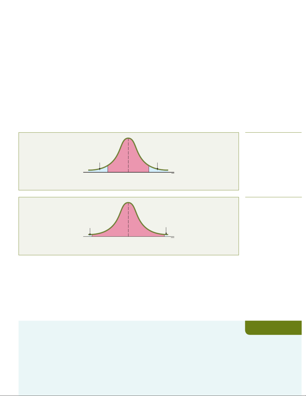
There is a different critical value for each level of confidence 1 - α. A level of confidence
of 95% leads to a Z value of 1.96 (see Figure 8.2). For a 99% level of confidence, α is 0.01. The
Z value is approximately 2.58 because the upper-tail area is 0.005 and the cumulative area less
than Z = 2.58 is 0.995 (see Figure 8.3). Figure 8.2 Normal curve for determining the Z value 0.025 0.025 needed for 95% confidence 0.475 0.475 μX –1.96 +1.960 Z Figure 8.3 Normal curve for determining the Z value 0.005 0.005 needed for 99% confidence 0.495 0.495 μ X –2.58 +2.58 0 Z
Now that various levels of confidence have been considered, why not make the confidence
level as close to 100% as possible? Before doing so, you need to realise that any increase in the
level of confidence is achieved only by widening (and making less precise) the confidence
interval. You would have more confidence that the population mean is within a broader range of
values. However, this might make the interpretation of the confidence interval less useful. The
trade-off between the width of the confidence interval and the level of confidence is discussed
in greater depth in the context of determining the sample size in Section 8.4.
Example 8.1 illustrates the application of the confidence interval estimate.
ESTIMATING THE MEAN SALMON WEIGHT WITH 95% CONFIDENCE EXAMPLE 8.1
Atlantic Salmon farming is an important industry in Tasmania. Fish are grown to market size in a
series of large, circular, netted enclosures in areas such as the Huon River, Port Esperance, the
D’Entrecasteaux Channel and around the Tasman Peninsula. When salmon are harvested to send to
market they need to weigh 3.5–4 kg, so the farmer is aiming to have an average weight of 3.75 kg.
We will assume that all salmon are placed in their final growing enclosure at the same time and
spend 12 months there, and that the standard deviation of their weights after that time is 380 g. A
farmer wishes to check whether the average weight of salmon in the enclosure falls in the required
range. He weighs a sample of 50 salmon being sent to market and finds their average weight is
3,607 g. Construct a 95% confidence interval estimate for the population mean salmon weight. 14:27, 11/01/2026
Confidence Intervals for Mean (σ Known): Chapter 8 Summary - Studocu SOLUTION
Using Equation 8.1 with Z = 1.96 for 95% confidence: σ 380 X ± Z = 3607 ± (1.96) 50 n = 3607 ± 105.33 3501.67 ⩽ μ ⩽ 3712.33
Copyright © Pearson Australia (a division of Pearson Australia Group Pty Ltd) 2019— 9781488617249 — Berenson/Basic Business Statistics 5e 14:27, 11/01/2026
Confidence Intervals for Mean (σ Known): Chapter 8 Summary - Studocu
284 CHAPTER 8 CONFIDENCE INTERVAL ESTIMATION
Thus, with 95% confidence you can conclude that the mean weight of salmon in the enclosure
is between 3,501.67 g and 3,712.33 g. This would indicate that the average weight of fish in
the enclosure is below the average of 3,750 g desirable for market-ready fish. We would
expect that many fish in the enclosure still need to grow larger before being harvested.
To see the effect of using a 99% confidence interval, examine Example 8.2. EXAMPLE 8.2
ESTIMATING THE MEAN SALMON WEIGHT WITH 99% CONFIDENCE
Construct a 99% confidence interval for the population mean salmon weight. SOLUTION
Using Equation 8.1 with Z = 2.58 for 99% confidence: σ 380 X ± Z = 3607 ± (2.58) n 50 = ± 3607 138.65 3468.35 ⩽ μ ⩽ 3745.65
The interval still does not contain the desired mean weight of 3.75 kg, so the fish will need to grow larger. Problems for Section 8.1 LEARNING THE BASICS
50 cans is selected, and the sample mean amount of paint per 8.1 If X
– = 85, σ = 8 and n = 64, construct a 95% confidence 4-litre can is 3.98 litres.
interval estimate of the population mean μ.
a. Construct a 99% confidence interval estimate of the 8.2 If X – = 125, σ = 24 and n = 36, construct a 99% confidence
population mean amount of paint included in a 4-litre can.
interval estimate of the population mean μ.
b. On the basis of your results, do you think that the manager
8.3 A market researcher states that she has 95% confidence that
has a right to complain to the manufacturer? Why?
the mean monthly sales of a product are between $170,000
c. Must you assume that the population amount of paint per
and $200,000. Explain the meaning of this statement.
can is normally distributed here? Explain.
8.4 Why is it not possible in Example 8.1 to have 100% confidence?
d. Construct a 95% confidence interval estimate. How does Explain.
this change your answer to (b)?
8.5 From the results of Example 8.1 regarding salmon farming, is it 8.8 The quality control manager at a light globe factory needs to
true that 95% of the sample means will fall between 3,501.67 g
estimate the mean life of a large shipment of energy-saving and 3,712.33 g? Explain.
light-emitting diode (LED) light globes. The standard deviation is
8.6 Is it true in Example 8.1 that you do not know for sure whether
3,000 hours. A random sample of 64 light globes indicates a
the population mean is between 3,501.67 g and 3,712.33 g?
sample mean life of 34,000 hours.
a. Construct a 95% confidence interval estimate of the 14:27, 11/01/2026
Confidence Intervals for Mean (σ Known): Chapter 8 Summary - Studocu Explain.
population mean life of light globes in this shipment. APPLYING THE CONCEPTS
b. Do you think that the manufacturer has the right to state that
8.7 The manager of a paint supply store wants to estimate the
the light globes last an average of 35,000 hours? Explain.
actual amount of paint contained in 4-litre cans purchased from
c. Must you assume that the population of light globe life is
a nationally known manufacturer. It is known from the normally distributed? Explain.
manufacturer’s specifications that the standard deviation of the
d. Suppose that the standard deviation changes to
amount of paint is equal to 0.08 litres. A random sample of
6,000 hours. What are your answers in (a) and (b)?
Copyright © Pearson Australia (a division of Pearson Australia Group Pty Ltd) 2019— 9781488617249 — Berenson/Basic Business Statistics 5e 14:27, 11/01/2026
Confidence Intervals for Mean (σ Known): Chapter 8 Summary - Studocu