Confidence Intervals for Mean with Unknown Standard Deviation môn Xác suất thống kê| Đại học Duy Tân

14:24, 11/01/2026
Confidence Intervals for Mean with Unknown Standard Deviation - Studocu
8.2 CONFIDENCE INTERVAL ESTIMATION FOR THE MEAN (σ UNKNOWN) 285
8.9 The inspection division of a state department that regulates trade
b. Must you assume that the population of soft-drink fill is
measurement wants to estimate the actual amount of soft drink in normally distributed? Explain.
2-litre bottles at the local bottling plant of a large, nationally
c. Explain why a value of 2.02 litres for a single bottle is not
known soft-drink company. The bottling plant has informed the
unusual, even though it is outside the confidence interval
inspection division that the population standard deviation for 2-litre you calculated.
bottles is 0.05 litres. A random sample of 100 2-litre bottles at this
d. Suppose that the sample mean had been 1.97 litres. What is
bottling plant indicates a sample mean of 1.99 litres. your answer to (a)?
a. Construct a 95% confidence interval estimate of the
population mean amount of soft drink in each bottle.
8.2 CONFIDENCE INTERVAL ESTIMATION FOR THE MEAN ( UNKNOWN) 𝛔
Just as the mean of the population μ is usually unknown, you rarely know the actual standard
deviation of the population, σ. Therefore, you need to develop a confidence interval estimate of – and S.
μ using only the sample statistics X Student’s t Distribution
At the beginning of the twentieth century a statistician for Guinness Breweries in Ireland (see
reference 1), William S. Gosset, wanted to make inferences about the mean when σ was
unknown. Because Guinness employees were not permitted to publish research work under
their own names, Gosset adopted the pseudonym ‘Student’. The distribution that he developed
is known as Student’s t distribution. Student’s t distribution
If the random variable X is normally distributed, then the following statistic has a t distribu- A continuous probability distribution
tion with n - 1 degrees of freedom: whose shape depends on the number of degrees of freedom. X − μ t = S degrees of freedom
Relate to the number of values in n
the calculation of a statistic that are free to vary.
This expression has the same form as the Z statistic in Equation 7.4 on page 254, except that S is
used to estimate the unknown σ. The concept of degrees of freedom is discussed further on page 286.
Properties of the t Distribution
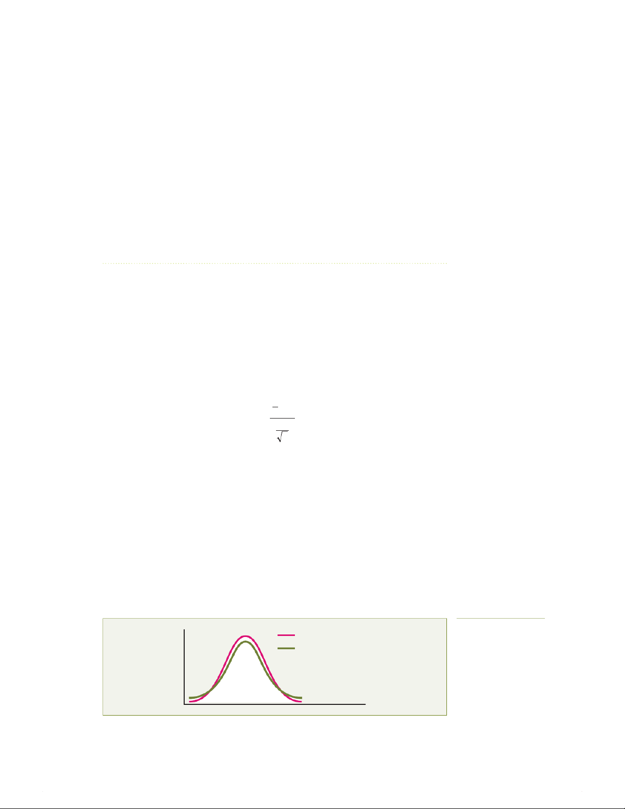
In appearance, the t distribution is very similar to the standardised normal distribution. Both
distributions are bell shaped. However, the t distribution has more area in the tails and less in
the centre than the standardised normal distribution (see Figure 8.4). Because the value of σ is
unknown and S is used to estimate it, the values of t are more variable than those for Z.
The degrees of freedom n - 1 are directly related to the sample size n. As the sample size
and degrees of freedom increase, S becomes a better estimate of σ and the t distribution gradu-
ally approaches the standardised normal distribution until the two are virtually identical. With a
sample size of about 120 or more, S estimates σ precisely enough that there is little difference
between the t and Z distributions. For this reason, most statisticians use Z instead of t when the
sample size is greater than 120. Figure 8.4 Standardised normal Standardised normal t distribution distribution and t for 5 degrees distribution for 5 degrees of freedom of freedom
Copyright © Pearson Australia (a division of Pearson Australia Group Pty Ltd) 2019— 9781488617249 — Berenson/Basic Business Statistics 5e 14:24, 11/01/2026
Confidence Intervals for Mean with Unknown Standard Deviation - Studocu
286 CHAPTER 8 CONFIDENCE INTERVAL ESTIMATION
As stated earlier, the t distribution assumes that the random variable X is normally distributed.
In practice, however, as long as the sample size is large enough and the population is not very
skewed, you can use the t distribution to estimate the population mean when σ is unknown. When
dealing with a small sample size and a skewed population distribution, the validity of the confi-
dence interval is a concern. To assess the assumption of normality, you can evaluate the shape of
the sample data by using a histogram, stem-and-leaf display, box-and-whisker plot or normal probability plot.
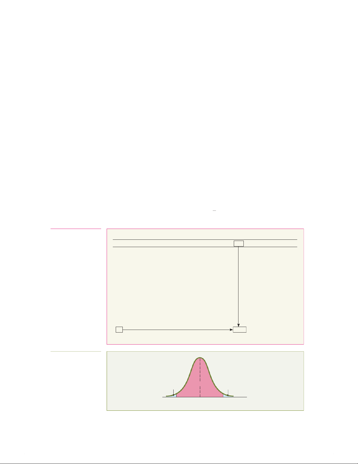
You find the critical values of t for the appropriate degrees of freedom from the table of the
t distribution (Table E.3). The columns of the table represent the area in the upper tail of the t
distribution. Each row represents the particular t value for each specific degree of freedom. For
example, with 99 degrees of freedom, if you want 95% confidence you find the appropriate
value of t as shown in Table 8.1. The 95% confidence level means that 2.5% of the values (an
area of 0.025) are in each tail of the distribution. Looking in the column for an upper-tail area
of 0.025 and in the row corresponding to 99 degrees of freedom gives you a critical value for t
of 1.9842. Because t is a symmetrical distribution with a mean of 0, if the upper-tail value is
+1.9842, the value for the lower-tail area (lower 0.025) is -1.9842. A t value of -1.9842 means
that the probability that t is less than -1.9842 is 0.025, or 2.5% (see Figure 8.5).
The Concept of Degrees of Freedom
In Chapter 3 we saw that the numerator of the sample variance S2 (see Equation 3.9a) requires the calculation of: n ∑(Xi − X)2 i = 1 Table 8.1 Upper-tail areas Determining the critical Degrees of freedom .25 .10 .05 .025 .01 .005 value from the t table for 1 1.0000 3.0777 6.3138 12.7062 31.8207 63.6574 an area of 0.025 in each 2 0.8165 1.8856 2.9200 4.3027 6.9646 9.9248 tail with 99 degrees of freedom 3 0.7649 1.6377 2.3534 3.1824 4.5407 5.8409 (extracted from Table E.3 in 4 0.7407 1.5332 2.1318 2.7764 3.7469 4.6041 Appendix E of this book) 5 0.7267 1.4759 2.0150 2.5706 3.3649 4.0322 . . . . . . . . . . . . . . . . . . . . . 96 0.6771 1.2904 1.6609 1.9850 2.3658 2.6280 97 0.6770 1.2903 1.6607 1.9847 2.3654 2.6275 98 0.6770 1.2902 1.6606 1.9845 2.3650 2.6269 99 0.6770 1.2902 1.6604 1.9842 2.3646 2.6264 100 0.6770 1.2901 1.6602 1.9840 2.3642 2.6259 Figure 8.5 t distribution with 99 degrees of freedom 1 – α = 0.95 0.025 0.025 –1.9842 t +1.9842 99
Copyright © Pearson Australia (a division of Pearson Australia Group Pty Ltd) 2019— 9781488617249 — Berenson/Basic Business Statistics 5e 14:24, 11/01/2026
Confidence Intervals for Mean with Unknown Standard Deviation - Studocu
8.2 CONFIDENCE INTERVAL ESTIMATION FOR THE MEAN (σ UNKNOWN) 287
In order to calculate S2, you first need to know X
–. Therefore, only n - 1 of the sample val-
ues are free to vary. This means that you have n - 1 degrees of freedom. For example, suppose
a sample of five values has a mean of 20. How many values do you need to know before you – = 20 also tells you that:
can determine the remainder of the values? The fact that n = 5 and X n Xi = 100 ∑ i = 1 because: n ∑Xi i = 1 = X n
Thus, when you know four of the values, the fifth one will not be free to vary because the sum
must add to 100. For example, if four of the values are 18, 24, 19 and 16, the fifth value must be 23 so that the sum equals 100.
The Confidence Interval Statement
Equation 8.2 defines the (1 - α) * 100% confidence interval estimate for the mean with σ LEARNING OBJECTIVE 1
unknown. Construct and interpret confidence intervals for the mean
CONFIDENCE INTERVAL FOR THE MEAN (σ UNKNOWN) S X ± tn−1 n or S S X − tn−1 ⩽ μ ⩽ X + tn−1 (8.2) n n
where tn-1 is the critical value of the t distribution with n - 1 degrees of freedom for an
area of α/2 in the upper tail.
To illustrate the application of the confidence interval estimate for the mean when the
standard deviation σ is unknown, return to the Callistemon Camping Supplies scenario pre-
sented on page 279. You select a sample of 100 sales invoices from the population of sales
invoices during the month and the sample mean of the 100 sales invoices is $230.27, with a
sample standard deviation of $52.62. For 95% confidence, the critical value from the t distribution
(as shown in Table 8.1) is 1.9842. Using Equation 8.2: S X ± tn−1 n 52.62 = 230.27 ± (1.9842) 100 = 230.27 ± 10.44 $219.83 ⩽ μ ⩽ $240.71
A Microsoft Excel worksheet for these data is presented in Figure 8.6 (overleaf).
Thus, with 95% confidence, you conclude that the mean amount of all the sales invoices
is between $219.83 and $240.71. The 95% confidence level indicates that if you selected all
possible samples of 100 (something that is never done in practice), 95% of the intervals devel-
oped would include the population mean somewhere within the interval. The validity of this
Copyright © Pearson Australia (a division of Pearson Australia Group Pty Ltd) 2019— 9781488617249 — Berenson/Basic Business Statistics 5e 14:24, 11/01/2026
Confidence Intervals for Mean with Unknown Standard Deviation - Studocu
288 CHAPTER 8 CONFIDENCE INTERVAL ESTIMATION Figure 8.6 A B Microsoft Excel 2016 1
Estimate for the mean sales invoice amount worksheet to calculate a 2 confidence interval 3 Data estimate for the mean 4 Sample standard deviation 52.62 sales invoice amount for 5 Sample mean 230.27 Callistemon Camping 6 Sample size 100 Supplies 7 Confidence level 95% 8 9 Intermediate calculations 10 Standard error of the mean 5.262 =B4/SQRT(B6) 11 Degrees of freedom 99 =B6 – 1 12 t value 1.984217 =T.INV .2T(1 – B7,B11) 13 Interval half width 10.44095 =B12 * B10 14 15 Confidence interval 16 Interval lower limit 219.8291 =B5 – B13 17 Interval upper limit 240.7109 =B5 + B13
confidence interval estimate depends on the assumption of normality for the distribution of the
amount of the sales invoices. With a sample of 100, the normality assumption is not overly restric-
tive and the use of the t distribution is probably appropriate. Example 8.3 further illustrates how to
construct the confidence interval for a mean when the population standard deviation is unknown. EXAMPLE 8.3
ESTIMATING THE MEAN HEIGHT OF FEMALE ATHLETES AGED 18–25
A manufacturer of women’s tracksuits needs to estimate the average height of female
athletes in the 18–25 age group. The measurements of a sample of 30 women are taken
and their heights recorded in millimetres. Table 8.2 lists these values. < HEIGHTS >
Construct a 95% confidence interval estimate for the population mean height of female athletes in this age group. Table 8.2
1,870 1,728 1,656 1,610 1,634 1,784 1,522 1,696 1,592 1,662 Heights (in millimetres)
1,866 1,764 1,734 1,662 1,734 1,774 1,550 1,756 1,762 1,866 of female athletes aged
1,820 1,744 1,788 1,688 1,810 1,752 1,680 1,810 1,652 1,736 18–25 SOLUTION
– = 1,723.4 mm and the sample standard devia-
Figure 8.7 shows that the sample mean is X
tion is S = 89.55 mm. Using Equation 8.2 to construct the confidence interv al, you need to
determine the critical value from the t table for an area of 0.025 in each tail with 29 degrees – = 1,723.4, S = 89.55, n = 30
of freedom. Table E.3 shows that t29 = 2.0452. Thus, using X and t29 = 2.0452: S X ± tn−1 n 89.55 = 1,723.4 ± (2.0452) 30 = 1,723.4 ± 33.44 1,689.96 ⩽ μ ⩽ 1,756.84
Copyright © Pearson Australia (a division of Pearson Australia Group Pty Ltd) 2019— 9781488617249 — Berenson/Basic Business Statistics 5e 14:24, 11/01/2026
Confidence Intervals for Mean with Unknown Standard Deviation - Studocu
8.2 CONFIDENCE INTERVAL ESTIMATION FOR THE MEAN (σ UNKNOWN) 289 A B Figure 8.7 1 One sample t: height PHStat confidence 2 interval estimate for the 3 Data mean height (in 4 Sample standard deviation 89.55083319 millimetres) of female 5 Sample mean 1723.4 athletes aged 18–25 6 Sample size 30 7 Confidence level 95% 8 9 Intermediate calculations 10 Standard error of the mean 16.34967046 11 Degrees of freedom 29 12 t value 2.045229642 13 Interval half width 33.43883066 14 15 Confidence interval 16 Interval lower limit 1689.96 17 Interval upper limit 1756.84
You conclude with 95% confidence that the mean height of 18–25-year-old female
athletes is between 1,689.96 and 1,756.84 mm. The validity of this confidence interval estimate
depends on the assumption that the heights in the population are normally distributed. Remember,
however, that you can slightly relax this assumption for large sample sizes. Thus, with a sample of
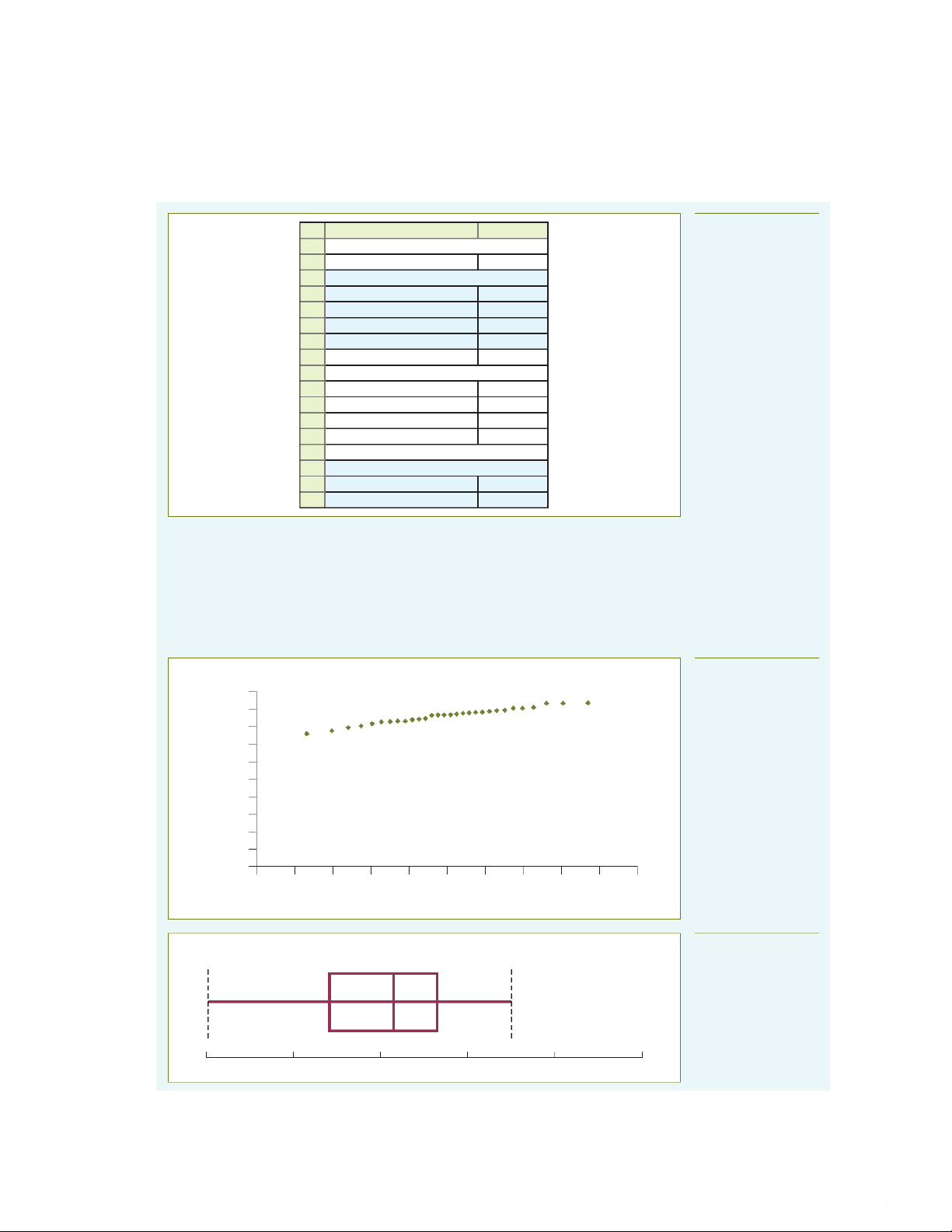
30, you can use the t distribution even if the distribution of heights is slightly skewed. From the
normal probability plot displayed in Figure 8.8, or the boxplot displayed in Figure 8.9, the heights
appear only slightly skewed. Thus the t distribution is appropriate for these data.
Normal probability plot of height Figure 8.8 2,000 PHStat normal probability 1,800 plot for the height (in 1,600 millimetres) of female 1,400 athletes aged 18–25 1,200 1,000 Height 800 600 400 200 0 –2 –2.5 –1.5 –1 –0.5 0 0.5 1.5 1 2.52 Z value Boxplot of height Figure 8.9 PHStat boxplot for the Height height (in millimetres) of female athletes aged 18–25 1,520 1,620 1,720 1,820 1,920 2,020
Copyright © Pearson Australia (a division of Pearson Australia Group Pty Ltd) 2019— 9781488617249 — Berenson/Basic Business Statistics 5e 14:24, 11/01/2026
Confidence Intervals for Mean with Unknown Standard Deviation - Studocu
290 CHAPTER 8 CONFIDENCE INTERVAL ESTIMATION
The validity of this confidence interval estimate depends on the assumption that the
processing time is normally distributed. What would happen if there was a small sample and
the boxplot and the normal probability plot indicted that the distribution was right-skewed?
In this case you would have some concern about the validity of the confidence interval in
estimating the population mean. The concern is that a 95% confidence interval based on a
small sample from a skewed distribution will contain the population mean less than 95% of
the time in repeated sampling. In the case of small sample sizes and skewed distributions,
you might consider the sample median as an estimate of central tendency and construct a
confidence interval for the population median (see reference 2). Problems for Section 8.2 LEARNING THE BASICS
8.16 Water resources in many parts of Australia are being closely
8.10 Determine the critical value of t in each of the following
watched and restrictions or water-wise rules have been circumstances:
imposed on activities such as garden watering. Suppose that a. 1 - α = 0.95, n = 10
Sydney Water monitors water usage in a suburb and finds that b. 1 - α = 0.99, n = 10
for one summer the average household usage is 408 litres per c. 1 - α = 0.95, n = 32
day. A year later it examines records of a sample of 50 d. 1 - α = 0.95, n = 65
households and finds that there is a daily mean usage of 380 e. 1 - α = 0.90, n = 16
litres with a standard deviation of 25 litres. –
8.11 If X = 75, S = 24, n = 36, and assuming that the population is
a. Construct a 95% confidence interval for the population
normally distributed, construct a 95% confidence interval
mean daily water usage in the second summer. Assume the
estimate of the population mean μ.
population usage is normally distributed. 8.12 If X
– = 50, S = 15, n = 16, and assuming that the population is
b. Interpret the interval constructed in (a).
normally distributed, construct a 99% confidence interval
c. Do you think water usage has changed in the second
estimate of the population mean μ. summer? Explain.
8.13 Construct a 95% confidence interval estimate for the population
8.17 The energy consumption of refrigerators sold in Australia and
mean, based on each of the following sets of data, assuming
New Zealand is checked and appliances are given a star rating
that the population is normally distributed:
to guide consumers who are about to make purchases. The Set 1: 1, 1, 1, 1, 8, 8, 8, 8
consumption in kilowatts per annum is also displayed for each Set 2: 1, 2, 3, 4, 5, 6, 7, 8
model on the website . Suppose a
Explain why these data sets have different confidence intervals
consumer organisation wants to estimate the actual electricity
even though they have the same mean and range.
usage of a model of refrigerator that has an advertised energy
8.14 Construct a 95% confidence interval for the population mean, based
usage of 355 kW per annum. It tests a random sample of
on the numbers 1, 2, 3, 4, 5, 6 and 20. Change the number 20 to 7
n = 18 fridges and finds a sample mean usage of 367 and a
and recalculate the confidence interval. Using these results, describe
sample standard deviation of 30.
the effect of an outlier (i.e. extreme value) on the confidence interval.
a. Assuming that the energy usage in the population is
normally distributed, construct a 95% confidence interval APPLYING THE CONCEPTS
estimate of the population mean energy usage for this model of refrigerator.
You can solve problems 8.15 to 8.21 with or without Microsoft Excel.
b. Do you think that the consumer organisation should accuse
8.15 A stationery store wants to estimate the mean retail value of
the manufacturer of producing fridges that do not meet the
greeting cards that it has in its inventory. A random sample of
advertised energy consumption? Explain.
20 greeting cards indicates a mean value of $4.95 and a
c. Explain why an observed energy usage of 350 kW standard deviation of $0.82.
for a particular refrigerator is not unusual, even
a. Assuming a normal distribution, construct a 95% confidence
though it is outside the confidence interval developed
interval estimate of the mean value of all greeting cards in in (a). the store’s inventory.
8.18 The data below represent the annual account fees for
b. How are the results in (a) useful in assisting the store owner
cheques made by a bank for a sample of 23 clients with
to estimate the total value of his inventory?
Copyright © Pearson Australia (a division of Pearson Australia Group Pty Ltd) 2019— 9781488617249 — Berenson/Basic Business Statistics 5e 14:24, 11/01/2026
Confidence Intervals for Mean with Unknown Standard Deviation - Studocu