DETAILED OUTLINE: MARKET STRUCTURES (MICROECONOMICS)
CHAPTER 13 – COSTS OF PRODUCTION
Firm’s objective: Profit maximization.
Profit formula: = TR − TC.π
Total Revenue (TR) = P × Q.
Explicit costs: direct monetary payments (wages, rent, materials).
Implicit costs: opportunity costs of owner-owned resources.
Total Cost (TC) = Explicit Costs + Implicit Costs.
Accounting profit = TR − Explicit costs.
Economic profit = TR − (Explicit + Implicit costs).
Production function: relationship between inputs and output.
Marginal Product of Labor (MPL) = Q / L.Δ Δ
Law of diminishing marginal product: MPL declines as L increases (fixed inputs).
Marginal Cost (MC) = TC / Q.Δ Δ
Fixed Cost (FC): does not vary with output.
Variable Cost (VC): varies with output.
Average Fixed Cost (AFC) = FC / Q.
Average Variable Cost (AVC) = VC / Q.
Average Total Cost (ATC) = TC / Q = AFC + AVC.
MC intersects ATC and AVC at their minimum points.
PERFECT COMPETITION
Characteristics: many buyers and sellers, homogeneous products, price takers, free
entry and exit.
Firm demand curve: P = AR = MR (horizontal).
Total Revenue (TR) = P × Q.
Average Revenue (AR) = TR / Q = P.
Marginal Revenue (MR) = TR / Q = P.Δ Δ
Profit maximization rule: MR = MC P = MC.⇒
Short run outcomes:
• Profit if P > ATC.
• Loss if AVC < P < ATC.
• Shutdown if P < AVC.
Shutdown condition: P < AVC.
Firm’s short-run supply curve: portion of MC above AVC.
Long-run decisions:
• Exit if P < ATC.
• Entry if P > ATC.
Long-run equilibrium: P = MC = min ATC.
Zero economic profit in the long run.
Perfect competition is allocatively efficient: P = MC.

MONOPOLY
Characteristics: single seller, no close substitutes, barriers to entry.
Demand curve: market demand, downward sloping.
Average Revenue (AR) = Demand.
Marginal Revenue (MR) lies below demand curve.
Reason: to sell more output, the monopolist must lower price on all units.
Profit maximization rule: MR = MC.
Price determination: P is taken from the demand curve at Q*.
Monopoly has no supply curve.
Short run: monopoly may earn profit or incur losses.
Long run: barriers to entry allow monopoly to earn positive economic profit.
Comparison with perfect competition: higher price, lower quantity.
Welfare loss: monopoly creates deadweight loss.
MONOPOLISTIC COMPETITION
Characteristics: many firms, differentiated products, free entry and exit.
Firm demand curve: downward sloping (product differentiation).
Average Revenue (AR) = Demand.
Marginal Revenue (MR) lies below demand curve.
Short run: profit maximization at MR = MC.
Short-run outcomes: firms may earn profit or incur losses.
If profits exist, new firms enter the market.
Long run: demand shifts left due to entry.
Long-run equilibrium: P = ATC.
Zero economic profit in the long run.
Firms do not produce at minimum ATC.
Excess capacity exists.
Market is not allocatively efficient: P > MC.
OLIGOPOLY
Characteristics: few dominant firms, interdependent decision-making.
Products may be homogeneous or differentiated.
No single standard model for oligopoly behavior.
Kinked demand curve model:
• Demand curve has a kink at current price.
• Marginal revenue curve is discontinuous.
Profit maximization: MR = MC within the discontinuous range.
Price rigidity: firms are reluctant to change prices.
Oligopolies often have significant barriers to entry.
Long run: firms may earn positive economic profit.
Market efficiency depends on competition versus collusion.
Bấm Tải xuống để xem toàn bộ.
Preview text:
DETAILED OUTLINE: MARKET STRUCTURES (MICROECONOMICS)
CHAPTER 13 – COSTS OF PRODUCTION
- Firm’s objective: Profit maximization.
- Profit formula: π = TR − TC.
- Total Revenue (TR) = P × Q.
- Explicit costs: direct monetary payments (wages, rent, materials).
- Implicit costs: opportunity costs of owner-owned resources.
- Total Cost (TC) = Explicit Costs + Implicit Costs.
- Accounting profit = TR − Explicit costs.
- Economic profit = TR − (Explicit + Implicit costs).
- Production function: relationship between inputs and output.
- Marginal Product of Labor (MPL) = ΔQ / ΔL.
- Law of diminishing marginal product: MPL declines as L increases (fixed inputs).
- Marginal Cost (MC) = ΔTC / ΔQ.
- Fixed Cost (FC): does not vary with output.
- Variable Cost (VC): varies with output.
- Average Fixed Cost (AFC) = FC / Q.
- Average Variable Cost (AVC) = VC / Q.
- Average Total Cost (ATC) = TC / Q = AFC + AVC.
- MC intersects ATC and AVC at their minimum points.
PERFECT COMPETITION
- Characteristics: many buyers and sellers, homogeneous products, price takers, free entry and exit.
- Firm demand curve: P = AR = MR (horizontal).
- Total Revenue (TR) = P × Q.
- Average Revenue (AR) = TR / Q = P.
- Marginal Revenue (MR) = ΔTR / ΔQ = P.
- Profit maximization rule: MR = MC ⇒ P = MC.
- Short run outcomes:
- • Profit if P > ATC.
- • Loss if AVC < P < ATC.
- • Shutdown if P < AVC.
- Shutdown condition: P < AVC.
- Firm’s short-run supply curve: portion of MC above AVC.
- Long-run decisions:
- • Exit if P < ATC.
- • Entry if P > ATC.
- Long-run equilibrium: P = MC = min ATC.
- Zero economic profit in the long run.
- Perfect competition is allocatively efficient: P = MC.
MONOPOLY
- Characteristics: single seller, no close substitutes, barriers to entry.
- Demand curve: market demand, downward sloping.
- Average Revenue (AR) = Demand.
- Marginal Revenue (MR) lies below demand curve.
- Reason: to sell more output, the monopolist must lower price on all units.
- Profit maximization rule: MR = MC.
- Price determination: P is taken from the demand curve at Q*.
- Monopoly has no supply curve.
- Short run: monopoly may earn profit or incur losses.
- Long run: barriers to entry allow monopoly to earn positive economic profit.
- Comparison with perfect competition: higher price, lower quantity.
- Welfare loss: monopoly creates deadweight loss.
MONOPOLISTIC COMPETITION
- Characteristics: many firms, differentiated products, free entry and exit.
- Firm demand curve: downward sloping (product differentiation).
- Average Revenue (AR) = Demand.
- Marginal Revenue (MR) lies below demand curve.
- Short run: profit maximization at MR = MC.
- Short-run outcomes: firms may earn profit or incur losses.
- If profits exist, new firms enter the market.
- Long run: demand shifts left due to entry.
- Long-run equilibrium: P = ATC.
- Zero economic profit in the long run.
- Firms do not produce at minimum ATC.
- Excess capacity exists.
- Market is not allocatively efficient: P > MC.
OLIGOPOLY
- Characteristics: few dominant firms, interdependent decision-making.
- Products may be homogeneous or differentiated.
- No single standard model for oligopoly behavior.
- Kinked demand curve model:
- • Demand curve has a kink at current price.
- • Marginal revenue curve is discontinuous.
- Profit maximization: MR = MC within the discontinuous range.
- Price rigidity: firms are reluctant to change prices.
- Oligopolies often have significant barriers to entry.
- Long run: firms may earn positive economic profit.
- Market efficiency depends on competition versus collusion.


