Economic Growth and Environmental Quality: Analysis of Government Expenditure and the Causal Effect
Báo cáo khoa học "Economic Growth and Environmental Quality: Analysis of Government Expenditure and the Causal Effect", tài liệu giúp sinh viên tham khảo và đạt điểm cao trong kỳ thi kết thúc môn!
Môn: Kinh tế vi mô (KTE201) 52 tài liệu
Trường: Trường Đại học Ngoại Thương 1.1 K tài liệu
Tác giả:


Preview text:
lOMoAR cPSD| 36066900 International Journal of Environmental Research and Public Health Article
Economic Growth and Environmental Quality: Analysis of
Government Expenditure and the Causal Effect
Mary Donkor 1,* , Yusheng Kong 1,*, Emmanuel Kwaku Manu 1, Albert Henry Ntarmah 1
and Florence Appiah-Twum 2 1
School of Finance and Economics, Jiangsu University, 301 Xuefu Road, Jingkou District, Zhenjiang 212013, China 2
School of Management, Jiangsu University, 301 Xuefu Road, Jingkou District, Zhenjiang 212013, China *
Correspondence: mdonkor34@gmail.com (M.D.); yshkong@ujs.edu.cn (Y.K.)
Abstract: Environmental expenditures (EX) are made by the government and industries which are
either long-term or short-term investments. The principal target of EX is to eliminate environmental
hazards, promote sustainable natural resources, and improve environmental quality (EQ). Thus,
this study looks at the impact of economic growth (EG), and government finance expenditure
(GEX) on EQ in Northern Africa and Southern Africa (NASA) republics from 2000–2016. The
panel quantile regression (PQR) and panel vector autoregressive (PVAR) model in a generalized
method of moment framework (GMM) were employed as a framework. The PQR results show that;
(i) In Northern republics, GEX had a significant positive effect on EQ at 25%, 50%, and 75% quantiles
levels. (ii) In the Southern republics, GEX had a significant negative impact on EQ at 25%. Moreover,
the PVAR through the GMM established that EG and GEX are significantly positive while the
parameter for CO2 is insignificant and negative in the North. However, in the South, GEX and
CO2 were statistically significant, while EG positively impacts EQ. Lastly, the granger causality
Citation: Donkor, M.; Kong, Y.;
report in North indicates uni-directional causation running from LNGEX → LNGDPpc, LNCO2 → Manu, E.K.; Ntarmah, A.H.;
LNGDPpc, LNFF → LNGEX, and LNFDI → LNGEX. Similarly, there is uni-directional causation in
Appiah-Twum, F. Economic Growth
South republics from LNGEX → LNGDPpc, LNCO2 → LNGEX, and LNFDI → LNGEX.
and Environmental Quality: Analysis
of Government Expenditure and the
Keywords: economic growth; government finance expenditure; environmental quality; panel
Causal Effect. Int. J. Environ. Res.
quantile regression; NASA republics
Public Health 2022, 19, 10629. https://doi.org/10.3390/ ijerph191710629 1. Introduction
Academic Editor: Daniela Varrica
Climate change and global warming are causing increasing harm, which has sparked Received: 17 June 2022
worldwide initiatives and partnerships to combat them through team efforts. The primary Accepted: 11 August 2022
cause of global warming is believed to be anthropogenic activities, namely the emissions of Published: 26 August 2022
greenhouse gases, mostly CO2 from the burning of fossil fuels such as oil, gas, and coal,
Publisher’s Note: MDPI stays neutral
deforestation, and untenable farming approaches which result from the rise in economic
with regard to jurisdictional claims in
activities. Economic activity is identified as the most important predictor of environmental
published maps and institutional affil-
degradation [1–3]. Expansion in economic activity means higher average income at the iations.
expense of natural resource depletion, hence, environmental degradation [4]. According
to the Classification of Environmental Protection Activities (CEPA 2000), environmen-
tal expenditure (EX) includes safeguarding sewage management, air and climate, waste
management, wildlife protection, R&D, bio-diversity groundwater, and land protection
Copyright: © 2022 by the authors.
expenses. EX refers to all spending to reduce the environmental hazards caused by the
Licensee MDPI, Basel, Switzerland.
processes above and improve environmental quality EQ [5]. EX is made by both the govern-
This article is an open access article
ment and private sectors and can be either short- or long-term expenditures. The primary
distributed under the terms and
conditions of the Creative Commons
objectives of these investments are to eliminate environmental harm, promote sustainable
Attribution (CC BY) license (https://
natural resource use, safeguard the environment and ameliorate EQ in general [6,7].
creativecommons.org/licenses/by/
According to the European Commission’s 7th Environment Action Programme assess- 4.0/).
ment, increasing EX in public and private sectors is crucial to enhancing EQ. In addition, lOMoAR cPSD| 36066900
Int. J. Environ. Res. Public Health 2022, 19, 10629 2 of 23
the initiatives produced within this context and the promotion of green technology are
said to reduce the harmful consequences of economic growth (EG) on the environment
and climate. Likewise, the reports state that the phenomena of EG and EQ will have a
favorable impact on each other, suggesting that EX in public and private sectors might
assure environmentally responsible growth by creating employment possibilities [8]. It is
critical to developing measures to avoid or mitigate environmental deterioration caused by
increased economic activity in light of these developments. As a result, the link between
EX and EQ is assessed regarding the size, content, and technical impact of spending. An
increase in EX in the context of public expenditures might promote EQ, yet a quantitative
increase in public expenditures may cause EQ to degrade due to the scale effect. In particu-
lar, government spending encouragement of labor-intensive sectors may help minimize
pollution caused by capital-intensive manufacturing processes as in rural electrification
using distributed photovoltaic systems (capital intensive) against wood-based home energy
(labor-intensive) [9]. The technical impact category of government finance expenditure
(GEX) which seeks to stimulate EQ, may be used to assess R&D efforts and investments in
the development of technology that does not degrade the environment [10,11]. EX is one
effective strategy for halting the steady deterioration of the environment.
Although the environment is seen as a fundamental component of society, it is ig-
nored in terms of GEX due to a lack of urgency in environmental conservation in Africa.
In general, most African economies do not prioritize or seek to achieve environmental
preservation as a goal, and there have been no uniform laws or regulations defining the
role of GEX in environmental preservation. However, the Paris Agreement built on the
UNFCC, recently observed (COP26) in Glasgow on 31 October–13 November 2021. One of
their goals was to bring all parties together in a common cause to reduce emissions that
negatively impact climate [12,13]. If EQ is deemed a luxury public benefit, Furuoka [14]
argues that then it should be given appropriate consideration if necessary public goods
are provided (water availability, health conditions, food security). This literature review
generates the idea that in economies with a substantial quantity of GEX, EQ must be given
significant consideration. Increasing GEX enhances environmental legislation, assists in
accelerating, and strengthens institutions working to champion EQ [15]. Pollution manage-
ment and EQ enhancement are dependent on the size of GEX’s environmental footprint and EQ requirements [16–18].
Economic development is critical for long-term progress, particularly in emerging
countries in NASA. Fincke and Greiner [19] argued that a high rate of EG is a key charac-
teristic of emerging market economies, and the residents’ quality of life and the country’s
economic progress are inextricably intertwined. In the broadest sense, it is claimed that
increasing economic activity such as production and consumption hastened the destruction
of the environment. Pyerina-Carmen [20] posited that lowering greenhouse gases such as
CO2 and supporting eco-friendly industrial and farming practices are a pivot to long-term
growth. Investment in education, infrastructure development, health and medical services,
agriculture, and the housing sector, encouraging local and foreign investments, eco-friendly
measures, and the proliferation of business-friendly policies, drive countries’ EG. Hence,
NASA republics can target these areas to boost the EG of their countries from the grassroots,
resulting in growth from the bottom to the top of the economic pyramid. Pollutants such as
CO2 are produced during industrial production and are one of the most significant causes
of environmental damage [1,21–23]. Rapid EG increases job prospects and income levels;
on the contrary, it reduces societal wellbeing by causing pollution and deterioration of the
environment, with natural resource destruction taking the lead. This research contributes
to the literature in the following ways:
Firstly, even though several studies on Africa in the area of EG-EQ have been con-
ducted [24–28] these researches have paid less attention to the GEX’s involvement in these
outcomes hence, the magnitude of GEX in maintaining environmental quality as coun-
tries pursue economic growth have yet not to be established in NASA economies. Thus,
this study is the first to use GEX, which adds to the current literature on the growth– lOMoAR cPSD| 36066900
Int. J. Environ. Res. Public Health 2022, 19, 10629 3 of 23
environment quality model in NASA economies. This helps to clarify the involvement of
the GEX dynamic inside the NASA republics framework for EG-EQ and whether there is a
causal relationship between EG, GEX, and EQ in these economies. Secondly, by looking at
the topic from the perspective of NASA republics, this research contributes to the regional
variations of NASA republics. According to the African literature, many studies focus on
Africa, as a region, socio-economic levels, or other sub-groups, with less emphasis on the
corresponding sub-regions. The evaluation intends to provide empirical facts for compar-
ison and specific area officials to make policy decisions by looking at the matters from
NASA’s perspective. Finally, when causal linkages between EG, GEX, and EQ established
from this study will help stakeholders to build effective policies and strategies for EG, GEX, and EQ in NASA republics.
Thirdly, in order to address issues of omitted variables biases (when variables of
significant impact are ignored) as suggested by Barreto [29], Clarke, and Wooldridge [30],
this study considered fossil fuel and FDI due to their significant contribution to growth
rate and environmental degradation. Fossil fuel is the primary energy generation in most
NASA economies and is an important determinant of economic growth. Reductions in
energy use through fossil fuels affect EG in adverse ways if EG causes energy use. The
discovery of Mensah et al. [27] in 22 selected republics in Africa suggested a long-term
and short-term bidirectional causal relationship between fossil fuel energy consumption
and EG. Moreover, findings from Baz et al. [31], and Gani [32] suggested fossil fuel is a
vital contributor to environmental quality degradation. Most multinational companies are
trooping into Africa due to its natural resources endowment and hence, FDI has increased
in SSA, studies by Ekwueme et al. [33], Vo and Zaman [34], Naz et al. [35], and Chenran
et al. [36] unearthed substantial impact of FDI to EG and environmental degradation.
Finally, contributing to the argument in Africa about the link between EG and EQ is
far from ended; per the limited research undertaken in this context, Aluko and Ibrahim [37]
investigated the link between EG and the technical influence of financial development on
EQ. Their study looked at the entire SSA countries whiles Gholipour and Farzanegan [11]
and Musah et al. [38] consider MENA and NA, respectively, due to their contribution
to global emissions. To fill this research gap, our study is the first of its kind in NASA
regions to use GEX from the perspective of sub-regional economies in Africa, which
provides a mean-based evaluation. In addition, it allows the series to be observed over time,
bolstering the ecological modernization theory, which asserts that innovative planning by
several economic managers can assist in distancing EG from ecological destruction [39]
and environmental protection activities. Hence this study looks at the relationship existing
between EG, GEX, and EQ in NASA economies.
The remaining portions of this report are organized as follows: part two summarizes
the literature that guided the investigation, and part three focuses on the study methods.
The study’s empirical outcomes are presented in part four, while the report’s conclusions
and policy implications are presented in the last section. 2. Literature Review
In this review, we evaluate the relationship between EG, GEX, and EQ. For clarity,
the literature review is divided into three sections—the overview of EQ-GEX, EG-GEX,
and EG-EQ. The next part will go through each nexus in detail, based on current and pertinent information.
2.1. Environmental Quality and Government Finance Expenditure
Considering the past research, the chosen nation and region groupings are identified,
and many environmental indicators such as ozone (O3), CO2, SO2, PM10, water quality,
and deforestation are all used. Even though there is no clear consensus on the impact
of public and EX on EQ, it is evident that EX has a beneficial impact on EQ in general.
However, the overall impact of EX on EQ is equivocal. Using panel data analysis Bernauer
and Koubi [40] examined the relationship between GEX and SO2 in 42 nations between lOMoAR cPSD| 36066900
Int. J. Environ. Res. Public Health 2022, 19, 10629 4 of 23
1971 and 1996. A positive association between GEX and SO2 was discovered in a study
that employed numerous political and economic aspects as a control variable. Accord-
ing to this finding, the air quality degrades as the size of the government grows in E G.
Lopez et al. [41], using panel data analysis, explored the links between public-goods ex-
penditure and water pollution. The study employed biological oxygen demand as a water
pollution indicator from 1980–2005 in 47 countries and SO2 and lead levels as air pollution
indicators between 1986–1999 in low- and middle-income nations. A statistically significant
negative connection was observed between expenditures, public goods, and pollution.
In addition, a non-significant link was discovered between total GEX and air and water
pollution. The result by Lin et al. [42] from their study on the spillover effect of EX on
pollution density for the period of 2005–2009 in 30 regions of China through panel data
analysis showed large investment expenditures caused a low level of pollution in high
technology growth in the environment with a spillover impact. The spillover impact of
EX was statistically significant and beneficial from the findings of this investigation. As a
result of the spillover effect, an increase in EX accelerates eco-technological advancement
and concluded from the study’s findings that there is a negative link between EX and pollution levels.
Moreover, Halkos and Paizanos [43] used panel data analysis to examine the direct
and indirect impacts of GEX on SO2 and CO2 for 77 nations. While the direct effect of GEX
on SO2 is statistically significant and negative in the 1980–2000 research, it was insignificant
for CO2. While GEX had a negative indirect effect in low-income areas, it was a favorable
indirect effect in high-income areas. Thus, the direct effect of GEX on SO2 and CO2 is
distinguished by the countries’ income levels. The study of Lopez and Palacios [44] uses
panel data analysis to look at the relationships between the total GEX ratio to GDP, the
share of good public expenditure in total spending, openness, and the impacts of the energy
levy on air pollution levels in Europe’s wealthiest 12 countries from 1995 to 2008. Air
pollution indicators included sulfur dioxide (SO2), nitrogen dioxide (NO2), and oxygen
(O3). The results showed a significant negative association between overall GEX and public
goods spending and SO2 and O3 emissions. Islam and Lopez [45] evaluated the impact of
public goods and social spending on air pollution, including EX by local and centralized
governments and state governments, for 51 US areas. The study proxied air pollution as
SO2, PM2.5, and O3 from 1983–2008. The results obtained from an unbalanced panel data
study suggested that centralized and local GEX reduces air pollution by 0.1 and 0.5 percent
for various contaminants. The spending of state administrations was shown to have little
impact on pollution. Per the findings, the content of spending was more essential than
the size of the public sector, particularly in the case of air pollution. Furthermore, it was
asserted that an upsurge in spending aimed at public and social places would improve air
quality, although overall, GEX remained the same.
Galinato and Galinato [46] investigated the impact of public goods spending on defor-
estation and CO2 from 1986–1999 for 12 countries. The imbalanced panel data demonstrated
a tangible link between public goods spending and deforestation and CO2. Nonetheless, the
association between total GEX and environmental indicators was significant and positive
in the short term but inconsequential in the long term. Gholipour and Farzanegan [11],
using panel data analysis, investigated the links between EX and air quality in 14 MENA
countries from 1996 to 2015. In the study, PM10 and CO2 were chosen as air quality mea-
sures. The variables of EX and air quality were shown to be cointegrated. However, EX
alone was not statistically significant. Nevertheless, it was shown that EX improved air
quality by considering organizational structure and governance quality. In a panel data
analysis of China’s most polluted seven cities from 2007 to 2015, He et al. [10] discovered a
long-term association between EX and air quality index. Per the results, EX and the total
air quality index have a favorable relationship. As a result, a 1% increase in EX across
the board would result in a 0.051% improvement in air quality. Additionally, assessing
individual cities’ results, an increase of 1% in EX would improve air quality by 0.078, 0.035,
0.097, and 0.091 percent in Beijing, Taiyuan, Chongqing, and Lanzhou, respectively. In the lOMoAR cPSD| 36066900
Int. J. Environ. Res. Public Health 2022, 19, 10629 5 of 23
cities of Shijiazhuang, Ji’nan, and Urumqi, although, there was no empirical influence of EX on air quality.
2.2. Economic Growth and Environmental Quality
Economic growth, as defined by upsurges in GDP, is the primary aim of macroeco-
nomic policymaking, particularly in capitalist nations that emerged after WWII [47]. The
“at what cost?” issue is frequently raised since continual GDP expansion is the desired
aim. Furthermore, what ecological and natural effects face in the name of EG is a source of
concern. Some studies outlined the significant impact of economic expansion on EQ. For
example, findings from Asongu et al. [3] studied on criticalities of growth and environmen-
tal sustainability suggested a significant positive impact of EG on EQ in African economies.
In addition, the study discovered a bidirectional causal linkage between EG and CO2 and
suggested the region promotes the need for a paradigm shift away from fossil fuels and
toward renewables. Studies by Ekwueme et al. [33] on the CO2 effect of renewable energy
utilization, fiscal development, and FDI in South Africa revealed no significant impact of
FDI on CO2 but a significant effect of GDP on CO2. Ssali et al. [2] and Mensah et al. [27],
established a positive influence of EG on SSA’s CO2.
Vo and Zaman [34] discovered EG and CO2 have a bidirectional relationship. The
causality findings substantially corroborate research that revealed a one-way directional
link between EG, CO2, and FDI, implying that dynamic correlations across metrics within
African countries are underappreciated. Naz et al. [35], Shoaib et al. [48], Sunkanmi et al. [49]
in Pakistan found a positive and substantial influence of FDI on CO2 in the long run.
Chenran et al. [36] discovered a significant short-term effect of FDI on CO2 emissions
in Laos. Using the ARDL approach, Hang and Ucal [50] examined the effect of FDI on
CO2 for Turkey and concluded that FDI has a considerable influence on CO2 emissions.
The outcome by Rehman et al. [51] suggested a downward trend in FDI to mitigate the
negative consequences of CO2 emissions. Furthermore, fluctuating expenditures have non-
eco-friendly effects and provide a positive relationship through CO2 emissions in the short
run. The findings also show that both positive and negative changes in FDI can damage
environmental eminence in the long run. Isik et al. [52], Isik et al. [53] findings on EG
development and EQ in the US state revealed a negative influence of fossil fuel consumption
in Texas, although it is known for oil-producing.
CO2 emissions are a significant source of worry across the world. However, the impact
on people’s quality of life and the environment varies by area and donates around 70% of
total GHG emissions [24,25]. Developed economies traditionally lead global CO2 emissions,
and emerging economies’ rapidly increasing energy consumption put their aggregate
emissions above the developed countries. In 2005, industrialized economies accounted for
over 40% of global CO2 emissions, developing nations for around 56%, and aviation and
maritime transport for the remaining 4% [54]. Africa economically lacks growth, wherein
21st-century electrification is still a problem and sticks to traditional biomass [25]. Although
economic growth is an ultimate focus, under the existing interregional trade policy, growing
recent economic activity in most African republics will result in considerable growth in
FDI, energy usage, GEX, and CO2 emissions by 2030 [55].
2.3. Economic Growth and Government Finance Expenditure
Keynesians believe that creativity and perilous processing of macroeconomic equi-
librium is built on economic indicators such as savings, consumption, national income,
and investment embedded in Keynesian growth theories [56]. According to Keynes, in an
environment with no market leverage, the government can interfere by enforcing macroe-
conomic policy to raise aggregate demand for revitalizing activities in an economy—for
example, using measures such as increasing GEX and decreasing taxes. Keynesians believe
that GEX quickens socio-economic development faster than monetary policy to expand
a country’s potential growth. Unquestionably, GEX is fundamental to every country’s
stability since the government’s ability to spend, and tax speeds up economic activities and lOMoAR cPSD| 36066900
Int. J. Environ. Res. Public Health 2022, 19, 10629 6 of 23
the general market environment. Some scholars investigated the relationship between GEX
and EG; however, the outcomes are quite disparate.
Bergh and Karlsson [57] examined government size as the part of tax over GDP and
concluded a negative linkage between it and EG. Using panel data from 30 OECD countries
from 1995–2014, Zimcik [58] found a negative association between government size and
EG. Contrarily, other studies claim a positive relation between GEX and EG. Jiranyakul [59]
investigated the impact of GEX on EG in Thailand and confirmed a positive relationship
between them. Tatahi et al. [60] explored panel data of 60 countries from 1976 to 2010 and
confirmed that achieving high EG is related to high GEX. Chandiol et al. [61] suggested
that the government of Pakistan should increase its expenditure on agriculture to improve
the national output in agriculture to induce EG. Khac and Tu [62] found that GEX increases
along with the development level of nations, and EG positively connects with investment.
Even though many varied findings are claimed, the effect of GEX on EG has been proven.
Findings by Isik [63] and Manu et al. [64] suggested that an increase in the GEX leads to a
rise in EG which subsequently influenced CO2 emissions.
The findings reported in the literature above demonstrate that there is widespread
debate on the EG-EQ relationship. By presenting GEX into the relationship of EG-EQ, this
study aims to determine the influence of EG, GEX on EQ and their causal effect. Thus, by
addressing omitted variable issues the study introduced FF and FDI as controlled variables
into this relation in the context of NASA republics, thereby expanding the current literature on EG-EQ. 3. Data and Variables
This study used panel data of Northern and Southern economies (Algeria, Egypt,
Libya, Morocco, Sudan, Tunisia, Angola, Botswana, Namibia, South Africa, Zambia, and
Zimbabwe) to research the relationship and causal effect of economic growth, government
finance expenditure and environmental quality, from 2000–2016, integrating fossil fuel
consumption (FF) and foreign direct investment (FDI). Since environmental issues are
becoming more prominent in these economies, attracting the attention of international
agencies [65,66]. Information on the factors mentioned above is carried out from the WDI of
the World Bank. Table 1 displays the scheme of the index information, while measurements
of connection of different factors incorporated in the series data of the study are outlined.
EG is essential to sustainable advancement, particularly in emerging economies. Fincke
and Greiner [19] argued that a high rate of EG is a crucial characteristic of emerging
market economies. The residents’ quality of life and the country’s economic progress are
inextricably linked. Pyerina-Carmen [20] recommended that decreasing carbon emissions
and encouraging environmentally-friendly industrial and farming techniques are crucial
to a long-term growth rate. CO2 is used as a proxy for EQ by Halkos and Paizanos [18],
Musah, et al. [26], Vo and Zaman [34], Chenran et al. [36], and Yaduma et al. [67] and is
a pollutant produced by burning fossil fuels, manufacturing cement, and utilizing solid,
liquid, and gas fuels, as well as gas flaring. The research contributes to the discussion
of regional disparities in growth and ecological effects and geographic variability in the
field [68] and the possible endogeneity problems raised in numerous studies [69]. Certain
SSA countries were taken out of the analysis due to a lack of data or inadequate data
across the sample period. To increase numerical accuracy, simulate improbability, and
eliminate endogeneity glitches, we used a list of potential rheostat indicators identified in
the literature to adjust for EG (based on early inquiry assessments). This is in line with the
recent study by Musah et al. [26], Ahmad et al. [69], and Bekhet et al. [70], on the crucial
role these components play in the growth and the environment. lOMoAR cPSD| 36066900
Int. J. Environ. Res. Public Health 2022, 19, 10629 7 of 23
Table 1. Variable definition. Var. Indicators Index (Code) Source
The aggregate gross value added to the economy by all
domestic manufacturers, plus any product tariffs, minus any Economic growth GDPPC
subsidies not included in the product value. It is estimated WDI (2020)
without considering the depreciation of manufactured assets
or natural resource depletion and deterioration.
Transfer payments, which include wage transfers (pension, Government finance GEX
social benefits) and capital transfers, along with expenditure, WDI (2020) expenditure
such as government expenditure and investment
Pollutants are produced by the combustion of fossil fuels, the Environmental CO2
manufacture of cement, the use of solid, liquid, and gaseous World Bank (2020) quality (EQ) Fossil fuel fuels, and also gas flaring.
Investing in commercial interests in a different country by Foreign direct
people or companies in another country. In other terms, FDI is FDI
an investment by a foreign entity in the form of controlling World Bank (2020) investment
ownership in a firm in another nation. Foreign direct investment (% of GDP)
To comprehend variances in growth and environmental consequences among NASA’s
regional blocks, descriptive statistics on a regional basis are presented. This can also
be used as a reference point for understanding data disparities. North Africa generates
the most significant carbon dioxide (M = 10.388, SD = 1.222), whereas South Africa pro-
duces the least (M = 8.955, SD = 1.770), according to Table 2. This indicates that North
Africa pollutes the African climate more than South Africa on average. Similarly, North
Africa recorded a high growth rate of (M = 8.535, SD = 0.517) than South republics of
(M = 8.250, SD = 0.954). Interestingly, North republics that produce high CO2 correspond
to the economic development rate, and the South that produces less CO2 has an average
growth out. As illustrated in this summary, NASA’s development and ecological outcomes
vary depending on its regional economic and ecological blocks. The authors restricted
NASA countries to their different economic and political features to prevent misleading
results when investigating this question. The data on kurtosis in the North are mostly
mesokurtic (kurtosis values of approximately 3). Except for FDI, the statistics in South
Africa have a mesokurtic structure. Apart from CO2 and GDPpc, the statistic in North-
ern Africa is leptokurtic (kurtosis value > 3). The JB and likelihood findings back up
Table 2’s informative statistics, which show that the data are normally distributed. In such
a distribution, heterogeneous panel data are ideal for researching the issue [27].
Table 2. Descriptive statistics. North South GDPpc GEX CO2 FF FDI GDPpc GEX CO2 FF FDI Mean 8.535 2.461 10.388 4.026 0.763 8.250 2.697 8.955 3.889 0.831 Median 8.569 2.556 10.350 4.205 0.765 7.814 2.683 8.273 4.386 1.160 Maximum 9.284 3.019 12.288 4.589 2.253 9.882 3.267 13.128 4.597 2.716 Minimum 7.723 −0.051 8.278 2.763 −1.660 6.956 1.937 7.119 1.801 −3.218 Std. Dev. 0.517 0.539 1.222 0.575 0.784 0.954 0.308 1.770 0.862 1.127 Skewness −0.074 −2.359 −0.078 −0.880 −0.472 0.273 −0.264 1.578 −1.042 −1.038 Kurtosis 1.569 9.950 1.731 2.452 3.942 1.394 2.506 4.146 2.432 3.765 Jarque–Bera 8.794 299.962 6.952 14.451 7.569 14.25 2.595 55.927 23.151 24.286 Probability 0.012 0.000 0.031 0.000 0.022 0.000 0.273 0.000 0.000 0.000 Sum Sq. Dev. 26.969 29.403 150.982 33.404 62.167 107.470 11.248 369.7544 87.831 150.064 Observations 102 102 102 102 102 119 119 119 119 119 lOMoAR cPSD| 36066900
Int. J. Environ. Res. Public Health 2022, 19, 10629 8 of 23 3.1. Preliminary Analysis 3.1.1. Trend of Variables
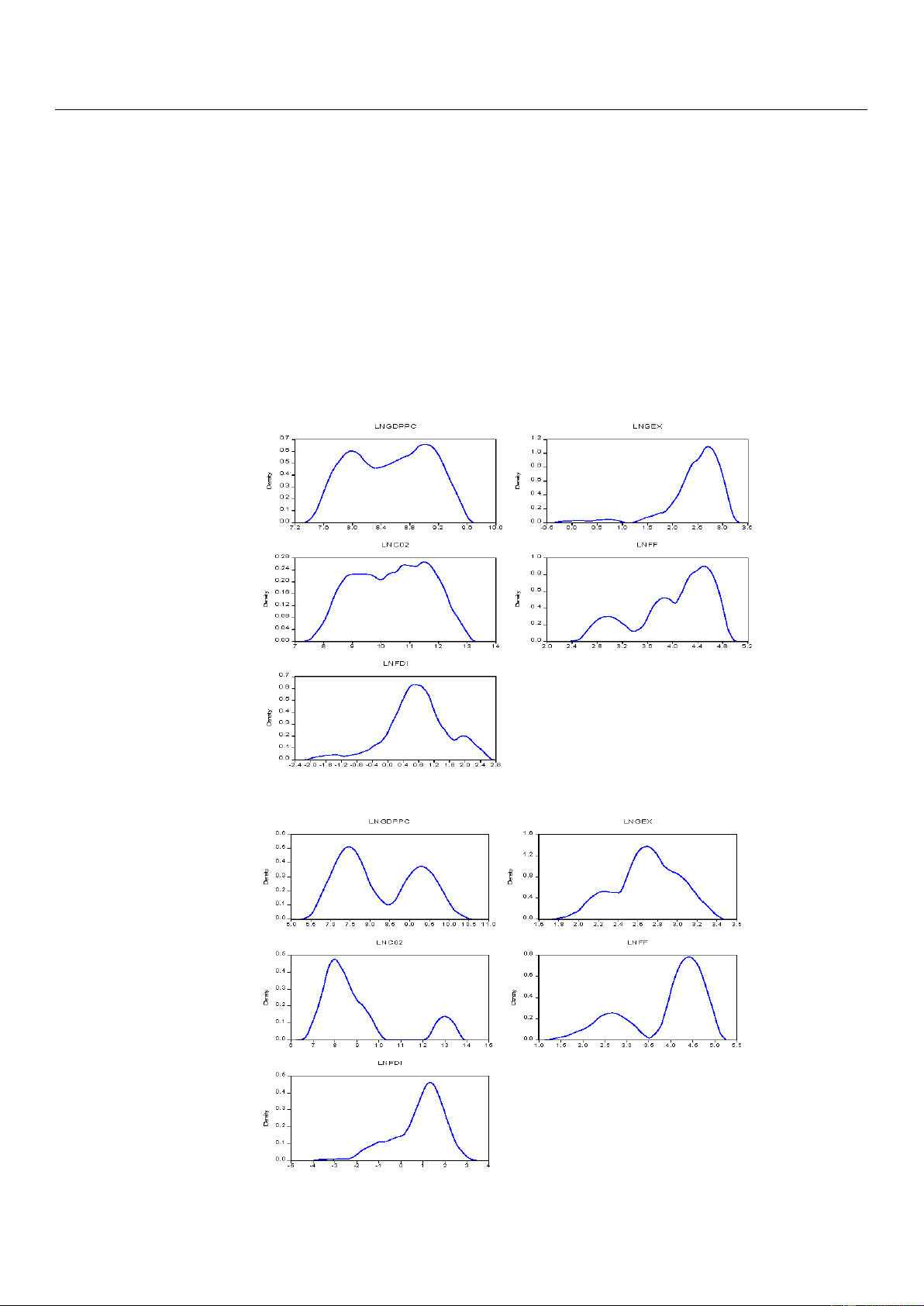
Kernel density distribution estimation is used in the study to explore the strength
of association amid the parameters. The trend of the study variables for the sub-regional
blocks is depicted in Figures 1 and 2. We can observe general trends of each variable in
two sub-regions. In the case of Northern, in general, we can observe an upward trend of
per capita GDPpc and CO2 emissions within the initial state although GDPpc dropped and
CO2 increased even though there were fluctuations. GEX was gradual but began to rise
but got to its peak of one and there was a decline over the period. FDI and FF gradually
increased over time but FF had a lot of up and downwards turnover time as compared to
FDI which had a smooth rise but decline over time as it hit its peak of 0.6. In the Southern
republics, it is observed that GDPpc and CO2 fluctuate in the same sequence over time.
GEX, FF, and FDI showed a gradual upward increment as well.
Figure 1. The trend of the indicators-North.
Figure 2. The trend of the indicators-South. lOMoAR cPSD| 36066900
Int. J. Environ. Res. Public Health 2022, 19, 10629 9 of 23
3.1.2. Cross-Sectional Dependency and Correlation Analysis
The CD test and the correlation coefficient are reported in Table 3. It is confirmed that
both the CDP-test and the CDLMadj test are used to analyze indicators to see if panel data
have cross-sectional conditions. The null hypothesis of cross-sectional independence for all
the metrics GDP, GEX, CO2, FF, and FDI is rejected at 1 percent [71,72]. As a result, panel
data with the parameter estimate exhibit cross-sections, according to this hypothesis.
Table 3. Cross-sectional dependency and correlation analysis.
Cross-Sectional Dependence Test North South CD Var. CD LMadj CD P Test p-Value p-Value CD LMadj P-Test p-Value p-Value Test Test GDPpc 15.124 *** 0.000 38.880 *** 0.000 12.879 *** 0.000 33.100 *** 0.000 GEX 3.035 *** 0.002 5.775 *** 0.000 −1.760 ** 0.078 8.780 *** 0.000 CO2 10.710 *** 0.000 21.917 *** 0.000 15.927 *** 0.000 36.129 *** 0.000 FF 2.603 *** 0.001 4.361 *** 0.000 5.637 *** 0.000 7.823 *** 0.000 FDI 4.395 *** 0.000 308.997 *** 0.000 4.239 *** 0.000 3.329 *** 0.000 Correlation-North Correlation-South LNGDPpc 1 1 LNGEX 0.305 1 0.586 1 LNCO2 0.693 −0.244 1 0.435 0.366 1 LNFF 0.5724 0.708 0.084 1 0.307 −0.107 0.033 1 LNFDI 0.0146 0.021 −0.147 0.067 1 −0.095 −0.056 −0.345 0.175 1
Note: ***, ** shows the rejection of the null hypothesis at 1% and 5% significance: the CD — P the test of Pesaran 2004 and CDLMadj.
Table 4 displays the significance level of the Pesaran unit root test, Johansen and
Westerlund’s long-run co-integration among LNGDPpc, LNGEX, LNCO2, LNFF, and
LNFDI in Africa. These findings back up the null hypothesis of no co-integration. In
addition, the Johansen co-integration test is used, which yields the same results as the
Westerlund test. This result suggests that the method used is compelling and intense,
implying that the succeeding process is economically substantial and reliable.
Table 4. Cointegration test. North South Pedroni Statistic Prob. Statistic Prob. Statistic Prob. Statistic Prob. Panel −0.663 0.746 0.191 0.424 −0.308 0.621 −0.104 0.541 v-statistic Panel 0.677 0.751 0.732 0.768 0.502 0.692 1.164 0.877 rho-statistic Panel −1.737 ** 0.041 −2.115 0.017 −3.715 *** 0.000 −2.442 ** 0.007 PP-statistic Panel −0.288 ** 0.086 −0.645 0.259 −2.256 ** 0.012 −3.568 *** 0.000 ADF-statistic
Alternative hypothesis: individual AR coefs. (between-dimension) Statistic Prob. Statistic Prob. Group 0.954 2.397 0.991 rho-statistic 1.694 Group −5.363 ** 0.000 −2.010 0.022 PP-statistic Group −0.683 ** 0.047 −4.104 *** 0.000 ADF-statistic lOMoAR cPSD| 36066900
Int. J. Environ. Res. Public Health 2022, 19, 10629 10 of 23 Table 4. Cont. North South Pedroni Statistic Prob. Statistic Prob. Statistic Prob. Statistic Prob. Kao Kao ADF t-Statistic Prob. ADF t-Statistic Prob. −1.561 * 0.059 −0.928 ** 0.076 Johansen Johansen Hypothesized Fisher Stat. * Fisher Stat. * Hypothesized Fisher Stat. * from the (from trace No. of CE (s) Prob. max-eigen Prob. test) test) None 110.5 0.000 110.5 0.000 77.84 0.000 77.84 0.000 At most 1 190.7 0.000 140.0 0.000 186.5 0.000 111.1 0.000 At most 2 95.67 0.000 57.01 0.000 105.7 0.000 70.05 0.000 At most 3 57.26 0.000 50.56 0.000 55.69 0.000 39.44 0.000 At most 4 23.94 0.020 23.94 0.020 44.27 0.000 44.27 0.000
Note: *, **, and ***, represent the statistical significance at 1% and 5%, and 10% levels, this represents the rejection
of the H:0 at 1% and 5%, and 10% levels of significance. 3.2. Model Estimation
This paper aims to assess the influence of EQ on EG in NASA nations, considering
the influence of GEX. To respond to the research quest, five indicators-economic growth,
government finance expenditure, carbon emission, fossil fuel and foreign direct investment
were evaluated. According to the growth impact, GDPpc improves EG by encouraging
investment activities, which promote per capita income, decline energy concentration,
and expands the environment by reducing CO2 [73,74]. As a result, we use the modified
Cobb–Douglas production function in this study: Y ∗
it = Ait f (Kit,Lit) (1)
where Yit is the output of countries i at time t, Ait is the Hicks technological factor, Kit
signifies capital quantified as the PKS, and Lit is the labor. The Cobb–Douglas is a produc-
tion approach that is widely used as an apt tool to find relations between production and economic factors: Y ∞ β it = Ait Kit Lit (2)
where ∞ and β are the elasticities of Y vis-à-vis L and PKS. Therefore, from the extended
Cobb–Douglas production function, it is assumed that the levels of government finance
expenditure [17,18,75] capital Kit = GEXit in the model, which includes CO2 proxying EQ, which is extended as: Y δ β γ
it = Ait GEXit Lit CO2it (3)
where CO2it and GEXit of country i and time t in years. Here δ and γ are the elasticities
of output. Taking the natural logarithm and dividing both sides of Equation (3), we have
panel data under per capita terms by the population. Meanwhile, the effect of labor is kept
unchanged, and we add fossil fuel and FDI as control variables. We now get a log-linear
version of the production function as follows:
ln Yit = ln Ait + δGEXit + γCO2it + σFFit + τFDIit (4) lOMoAR cPSD| 36066900
Int. J. Environ. Res. Public Health 2022, 19, 10629 11 of 23
where lnAit = β0 + εit with β0 measuring the mean efficiency level across cross-sections
and overtime while εit is the country-specific deviations from the mean. Equation (4) can
be written in the following form:
ln Yit = β0 + δGEXit + γCO2it + σFFit + τFDIit + εit (5)
In the previous model, Yit is the response variable representing GDPpcit, GEXit, CO2it
FFit, and FDIit as explanatory variables. Therefore, the study attempts to calculate the PK
corresponding to the individual countries within the panel. The linear relation between EG
and EQ can be expressed as follows:
ln GDPpcit = f (ln GEXit, ln CO2it, ln FFit, ln FDIit) (6)
The forecast model’s empirical design is affirmed as:
ln GDPpcit = β0 + β1GEXit + β2CO2it + β3FFit + β4FDIit + εit (7)
∆ ln GDPpcit = µ1i + ∑p β1j ∆ ln GEXit−j + ∑p φ1j ∆ ln CO2it−j + ∑p ϕ ∆ 1j ln FFit−j j=1 p j=1 j=1 (8) +∑ γ∆ j=1
ln FDI+α1i + δ1t + ε1it
Environmental research frequently uses quantile regression, which has recently
emerged as a major area of study because the normalcy evaluation uncovers information
that isn’t commonly recognized, the model predisposes OLS by restricting such measures.
In such instances, the regression takes into account the findings of various percentiles
of dispersion and varied responses. Many contacts to be regulated by OLS and another
outmoded econometric approach were overlooked by regression projection for the intensity
of the irregularity and the capacity to tighten greatly. We employ the PQR approach of
Fan et al. [76] which is used to assess outcomes based on present conditions that exist
irrespective of everyone’s capacity or to create presumptions circulation [77–79]. The
controlled percentile was evaluated as QY(τ|X) a situation quantified in the form:
Qτ(ln GDPpcit) = ατ + β1τ ln GEXit + β2τ ln CO2it + β3τ ln FFit + β4τ ln FDIit + εit (9)
Equation (10) represents the PQR Equation of GDPpc depending on fixed effects (ατ),
GEX, CO2, FF, and FDI, where Qτ indicates the QR components of the τth differential point
that posits the differential point for the predictor variables. To address endogeneity issues,
the lagged evaluated measures were employed in Equation (10) [39,80].
Again, Pedroni, Kao, and Johansen’s co-integration show that variables are integrated
in the order I(0) and I(1), and the PVAR model is employed. The most crucial source
of macroeconomic dynamics in an open economy is endogenous and exogenous shocks,
which are modeled by the PVAR. The PVAR model has no bias against any particular
theories of economic expansion. The PVAR model, in contrast to VAR, adds to the dynamic
heterogeneity of our data, enhancing measurement of consistency and coherence, partic-
ularly where there is heterogeneity in GDP per capita, CO2 emissions, GEX, FF, and FDI
among NASA republics. Conferring to Love and Zicchino [80], the procedure for PVAR is as follows:
Yit = µi + A(L)Yit + αi + δt + εit (10)
i = 1, 2, 3 . . . N t = 1, 2, 3 . . . T.
4. Results and Discussion
The quantile regression results in Table 5 demonstrate that conditioning on other
determinants of GEX on EQ had a substantial positive impact at all levels of quantiles in the
Northern republics. However, the marginal effect rises at 1% from lower to higher quantile.
As a result, if all other parameters remain equal, a 1% rise in the GEX will result in an
11.4 percent increase in EQ spending, from a low growth rate of (25th quantile) to a high lOMoAR cPSD| 36066900
Int. J. Environ. Res. Public Health 2022, 19, 10629 12 of 23
growth rate of (25th quantile) (75th quantile). According to the findings, nations on a high-
growth road are more likely to benefit from boosting the GEX than those on a low-growth
path. CO2 emission has no significant impact on growth and EQ. FF consumption has a
positive and significant impact from the lower quantile to the highest quantile.
Table 5. Quantile regression. North South ALL 25% 50% 75% 25% 50% 75% 0.535 *** 0.114 *** 0.097 *** 0.081 * −0.215 * −0.118 −0.046 LNGEX (0.092) (0.037) (0.026) (0.033) (0.403) (5.927) (10.069) 0.247 *** −0.096 −0.068 −0.042 −0.0228 0.044 0.093 LNCO2 (0.025) (0.071) (0.050) (0.063) (0.357) (5.243) (8.906) 0.276 *** 0.345 *** 0.347 *** 0.349 *** 0.202 0.131 0.077 LNFF (0.056) (0.098) (0.069) (0.088) (0.417) (6.115) (10.387) 0.030 LNFDI 0.018 * 0.014 * 0.010 0.003 0.000 −0.001 (0.043) (0.009) (0.007) (0.008) (0.052) (0.767) (1.303) 3.507 *** 0.026 *** 0.026 *** 0.026 *** 0.022 0.020 0.018 Year (0.370) (0.003) (0.002) (0.002) (0.016) (0.234) (0.397)
*** and * indicate significant at 1% and 10% levels, respectively. Standard errors are in parenthesis.
Interestingly, an increase in FF increases EQ by 34.5%, 6.9%, and 34.9%. Last, FDI has
a positive and significant effect on EQ. All other things being equal FDI increases from the
lower quantile to the highest quantile. In the South, GEX had a negative and significant
impact on EQ, meaning that GEX on the environment is minimal and has no impact on
EQ. The other determinants (CO2, FF, and FDI) of EQ in the South are reported to have no impact on the environment.
We use a graphical methodology to emphasize the marginal effects of GEX on the EG
of economies at different growing levels to prove further the acceptability of employing
the quantile regression method over the OLS method. Using quantile regression and OLS
results, the effects of GEX efficiency on EG are visually illustrated in Figures 3 and 4. The
coefficients surrounding the quantile estimates (green line or a gray area in confidence
interval term) fluctuate dramatically with the diverse quantiles of EG. In contrast, the
OLS approach (dotted line) remains static in the chosen quantiles. Because the quantile
regression evaluations provide varying outcomes at different distributive locations on
the graph, it is evident that utilizing OLS estimations to create a constant estimate for all
economies would result in biased estimations because it does not justify outliers, as seen
in Figures 3 and 4. As a result, the quantile graph proves the suitability of the quantile regression approach over OLS. Figure 3. PQR-North. lOMoAR cPSD| 36066900
Int. J. Environ. Res. Public Health 2022, 19, 10629 13 of 23 Figure 4. PQR-South. 4.1. PVAR Results
The optimum lag for PVAR estimations, per Andrews and Lu [81], was among the
selected lag best three criteria: MQIC, MBIC, and MAIC. Hence, we employed the GMM
approach to applying the first-order lag PVAR model in its stationary version, as suggested
by Love and Zicchino [82] and adopted by Andrews and Lu [81]. The PVAR results are
shown in Table 6. In North Africa, the parameters of EG are positive and significant, while
the parameter for CO2 is negative and insignificant. Meaning that expansion in these
countries’ economies increases their CO2 emissions, thus, decreasing EQ, as stated by
previous studies by Ssali et al. [2] and Mensah et al. [27], who discovered that EG had a
substantial influence on SSA’s CO2 levels.
Interestingly, in South Africa, the parameter of EG is positive and significant, while
the parameter for CO2 is significant and negative. This can be explained as expansion in
nations’ economies grows, and increases CO2, hence improving EQ, but the growth of
improvement does not affect EQ. This supports the findings of Vo and Zaman [34] that
EG is positively related to CO2 and FDI, suggesting that GEX improves EQ in African
countries. Similarly, the parameter of GEX is positive and significant in the North, which
explains that GEX improves EG and EQ [10,44,46]. The parameter of GEX in the South
had a positive and insignificant outcome on EG and EQ. FDI in the Northern republics
positively and significantly affected EG and EQ. Moreover, the parameter of FDI had
a positive and insignificant outcome on growth and the environment. Our outcomes
support references [22,35,36,49,83], revealing FDI had a substantial impact on CO2 emis-
sions. FDI has historically been a trademark of globalization, assisting in transforming
whole companies, cities, industries, and economies. FDI has been a tried and tested
method for capital, technology, and transfer of better life throughout the world for decades.
Aside from increasing GDP through diversified businesses investment portfolios expan-
sion and lowering poverty, it stimulates innovations, knowledge sharing, modernized
business practices, and environmental protection. Nonetheless, the governments of host
nations have been drawn to the negative impact of FDI on their environment. They
have opted for high-quality investment that tackles EQ, climate change, and advanced sustainable development. lOMoAR cPSD| 36066900
Int. J. Environ. Res. Public Health 2022, 19, 10629 14 of 23
Table 6. PVAR style GMM results. LNGDPpc North South lngdppc L1. 0.853 *** 0.020 0.000 2.111 *** 0.233 0.000 lngex L1. 0.038 *** 0.007 0.000 −0.592 *** 0.114 0.000 lnco2 L1. −0.007 0.020 0.724 −0.533 *** 0.133 0.000 lnff L1. 0.278 *** 0.041 0.000 −0.058 0.075 0.442 lnfdi L1. 0.021 *** 0.003 0.000 −0.049 *** 0.009 0.000 lngex lngdppc L1. −0.978 *** 0.151 0.000 0.285 0.195 0.144 lngex L1. 1.219 *** 0.055 0.000 0.704 0.128 0.000 lnco2 L1. 0.283 0.166 0.089 −0.198 0.112 0.076 lnff L1. 1.776 *** 0.405 0.000 0.003 0.095 0.972 lnfdi L1. 0.065 ** 0.020 0.001 0.017 0.009 0.070 lnco2 lngdppc L1. −0.122 * 0.060 0.044 4.418 0.947 0.000 lngex L1. 0.042 * 0.019 0.026 −2.472 0.442 0.000 lnco2 L1. 0.945 *** 0.050 0.000 −1.136 0.528 0.032 lnff L1. 0.241 * 0.099 0.015 −0.379 0.298 0.204 lnfdi L1. 0.018 ** 0.006 0.001 −0.164 0.042 0.000 lnff lngdppc L1. 0.048 0.040 0.233 0.709 0.168 0.000 lngex −0.070 *** 0.009 0.000 −0.365 0.082 0.000 lnco2 L1. 0.101 ** 0.035 0.003 −0.317 0.094 0.001 lnff L1. 0.289 *** 0.067 0.000 0.759 0.062 0.000 lnfdi L1. −0.013 *** 0.003 0.000 −0.028 0.009 0.002 lnfdi lngdppc L1. −2.102 ** 0.823 0.011 17.475 3.713 0.000 lngex L1. 1.870 *** 0.293 0.000 −9.639 1.885 0.000 Lnco2 L1. −1.681 ** 0.765 0.028 −8.022 2.099 0.000 lnff L1. 15.946 *** 1.676 0.000 −0.884 1.381 0.522 lnfdi L1. 0.903 *** 0.155 0.000 −0.181 0.193 0.348
***, ** and * indicate significant at 1%, 5% and 10% levels, respectively.
4.2. Variance Decomposition
The VD is used to determine how much of the dependent indicator’s variation over
time can be explained by its latency and other descriptive indicators. The findings from VD
are summarized in Table 7. Because most of the components have the most control over
the others, we comprehend the results for the tenth period of this study. In North Africa,
evidence from Table 7 shows that LNGDPpc is explained by another determinant by 17%,
17%, 39%, 19.7, and 8.3% for the future variations due to shocks in LNGEX, LNCO2 LNFF,
and LNFDI. Moreover, 5.1%, 38.8%, 46.3%, 8.6%, and 1% of future fluctuation in LNGFE
are due to shocks in LNGDPpc, LNFF, and LNFDI. Moreover, 5.4%, 3.9%, 82.1%, 6.8%, and
1.9% of future fluctuation in LNFF are due to shocks in LNGDPpc, LNGEX, LNCO2, and
LNFDI. Furthermore, 9%, 7.9%, 2.2%, 73.5%, and 6.9% of future fluctuation in LNCO2 are
due to shocks in LNGDPpc, GEX, LNFF, and LNFDI. Lastly, 6.3%, 45.2%, 25.4%, 2.0%, and
3.1% of future fluctuation in LNFDI are due to shocks in LNGDPpc, LNCO2, LNFF, and
LNFDI, which support. Muhammed and Khan [84] concluded the positive influence of
FDI on CO2 for Asian economies. Economic growth is comparatively higher in value than
SE. Economic growth in the West confirms the ARDL results in Table 5 where the impact
of EG is greater than renewal energy accounting for (25.7%, and 85.4%). This implies that
when EG increases, the CO2 and FF impact is substantially minimal and thus improves the
environment, and requires less innovation and technology to control and manage energy
renewal which supports Ssali et al. [2] and Mensah et al. [27] who established positive impact of EG on SSA’s CO2. lOMoAR cPSD| 36066900
Int. J. Environ. Res. Public Health 2022, 19, 10629 15 of 23
Table 7. Variance decomposition results. LNGDPpc 1 1.000 0.000 0.000 0.000 0.000 1.000 0.000 0.000 0.000 0.000 2 0.842 0.024 0.007 0.006 0.121 0.723 0.074 0.157 0.000 0.046 3 0.678 0.055 0.025 0.051 0.192 0.795 0.057 0.112 0.000 0.036 4 0.539 0.082 0.055 0.114 0.209 0.718 0.064 0.163 0.000 0.055 5 0.430 0.105 0.097 0.170 0.197 0.751 0.059 0.140 0.001 0.050 6 0.348 0.123 0.149 0.207 0.173 0.704 0.058 0.176 0.001 0.061 7 0.285 0.136 0.208 0.223 0.147 0.721 0.058 0.163 0.001 0.058 8 0.237 0.147 0.270 0.224 0.122 0.687 0.055 0.193 0.001 0.064 9 0.200 0.154 0.331 0.213 0.101 0.693 0.058 0.185 0.002 0.062 10 0.170 0.160 0.390 0.197 0.083 0.665 0.054 0.212 0.002 0.067 lngex 0.000 0.000 0.000 0.000 0.000 0.013 0.987 0.000 0.000 0.000 1 0.173 0.827 0.000 0.000 0.000 0.034 0.927 0.028 0.000 0.012 2 0.190 0.758 0.019 0.015 0.017 0.028 0.902 0.037 0.000 0.033 3 0.177 0.686 0.059 0.048 0.031 0.048 0.853 0.053 0.001 0.045 4 0.152 0.621 0.113 0.080 0.035 0.045 0.838 0.056 0.001 0.060 5 0.126 0.566 0.174 0.102 0.032 0.058 0.811 0.061 0.002 0.068 6 0.104 0.519 0.239 0.112 0.026 0.057 0.802 0.060 0.003 0.078 7 0.086 0.479 0.302 0.112 0.021 0.065 0.786 0.061 0.004 0.084 8 0.072 0.445 0.362 0.106 0.016 0.065 0.780 0.059 0.005 0.091 9 0.060 0.415 0.416 0.096 0.013 0.071 0.769 0.058 0.006 0.096 10 0.051 0.389 0.463 0.086 0.010 0.013 0.987 0.000 0.000 0.000 lnco2 0.000 0.000 0.000 0.000 0.000 0.942 0.000 0.057 0.000 0.000 1 0.115 0.002 0.884 0.000 0.000 0.763 0.105 0.094 0.001 0.038 2 0.153 0.002 0.833 0.001 0.012 0.816 0.075 0.081 0.000 0.028 3 0.171 0.008 0.785 0.007 0.028 0.762 0.099 0.096 0.001 0.043 4 0.171 0.019 0.749 0.022 0.039 0.790 0.085 0.087 0.000 0.038 5 0.160 0.031 0.725 0.040 0.044 0.759 0.096 0.099 0.000 0.047 6 0.145 0.042 0.713 0.056 0.044 0.777 0.088 0.091 0.000 0.044 7 0.129 0.053 0.712 0.066 0.040 0.755 0.092 0.102 0.000 0.050 8 0.115 0.063 0.717 0.071 0.035 0.767 0.088 0.097 0.000 0.048 9 0.102 0.072 0.725 0.071 0.030 0.751 0.089 0.107 0.000 0.053 10 0.090 0.079 0.735 0.069 0.026 0.942 0.000 0.057 0.000 0.000 lnff 0.000 0.000 0.000 0.000 0.000 0.699 0.001 0.069 0.230 0.000 1 0.111 0.123 0.109 0.656 0.000 0.623 0.074 0.075 0.194 0.034 2 0.155 0.216 0.117 0.486 0.026 0.664 0.056 0.073 0.181 0.025 3 0.167 0.309 0.100 0.370 0.054 0.648 0.065 0.081 0.169 0.037 4 0.154 0.379 0.079 0.322 0.065 0.671 0.061 0.076 0.160 0.032 5 0.134 0.425 0.072 0.306 0.063 0.663 0.062 0.086 0.152 0.038 6 0.114 0.453 0.084 0.295 0.054 0.677 0.061 0.081 0.146 0.035 7 0.097 0.466 0.114 0.277 0.046 0.671 0.060 0.090 0.140 0.038 8 0.084 0.468 0.156 0.253 0.040 0.680 0.062 0.086 0.136 0.036 9 0.072 0.463 0.204 0.226 0.035 0.699 0.001 0.069 0.230 0.000 10 0.063 0.452 0.254 0.200 0.031 0.623 0.074 0.075 0.194 0.034 lnfdi 1 0.461 0.019 0.000 0.093 0.427 0.834 0.001 0.006 0.000 0.158 2 0.399 0.047 0.005 0.095 0.455 0.768 0.070 0.098 0.000 0.064 3 0.318 0.069 0.024 0.182 0.406 0.796 0.063 0.089 0.000 0.053 4 0.260 0.083 0.059 0.251 0.347 0.790 0.065 0.098 0.000 0.046 5 0.223 0.092 0.106 0.279 0.300 0.799 0.064 0.095 0.000 0.041 6 0.199 0.098 0.159 0.277 0.268 0.796 0.064 0.099 0.000 0.040 7 0.181 0.100 0.212 0.262 0.245 0.801 0.065 0.097 0.000 0.037 8 0.167 0.102 0.261 0.243 0.227 0.799 0.064 0.100 0.000 0.036 9 0.155 0.103 0.304 0.225 0.213 0.802 0.065 0.098 0.001 0.035 10 0.144 0.104 0.342 0.210 0.200 0.800 0.064 0.101 0.000 0.035 lOMoAR cPSD| 36066900
Int. J. Environ. Res. Public Health 2022, 19, 10629 16 of 23
In the South, the results show that 66.5%, 5.4%, 21.2%, 0.2%, and 6.7% of impending
fluctuations in LNGDPpc are due to shocks in LNCO2 LNFF LNGEX, and LNFDI. In
addition, 1.3% and 98.7% of future fluctuation in LNGEX are due to shocks in LNGDPpc.
Moreover, 94.2% and 5.7% of the future variation in LNFF are due to shocks in LNCO2.
Furthermore, 62.3%, 7.4%, 7.5%, 19.4%, and 3.4% of future fluctuation in LNFDI are due to
shocks in LNGDPpc, LNCO2, LNFF, and LNFDI [34,36].
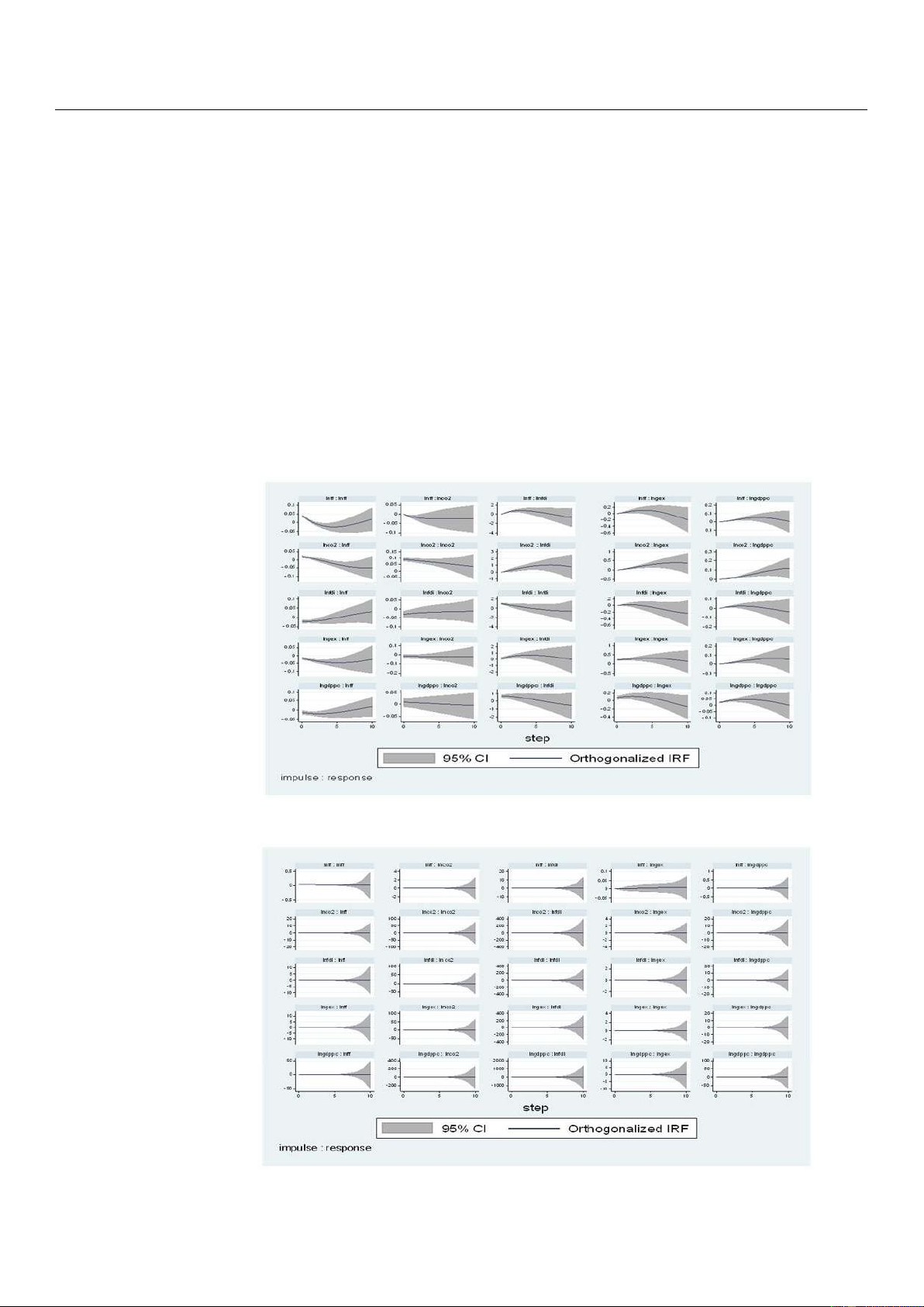
4.3. Impulse Response Analysis (IRA)
The (IRA) is used in this study to look at how LNGDPpc, LNGEX, LNCO2, LNFF, and
LNFDI react to random changes in each other that are not clarified by the Granger causatives
test. The (IRA) avoids the orthogonal pitfalls that out-of-sample Granger causality tests are
prone to. Figures 5 and 6 show the LNGDP (IRA) to Cholesky One SD. Innovations in other
factors. In North Africa, confirmation from Figure 5 displays that the reaction of LNGDP
to innovation is significant within the 4-period limit. The initial response of LNGDPpc
to LNGEX, LNCO2, LNFF, and LNFDI is positive and significant, which supports [35] in
Pakistan, disclosed a positive effect from FDI to CO2 in the long run. Figure 5. IRF-North. Figure 6. IRF-South. lOMoAR cPSD| 36066900
Int. J. Environ. Res. Public Health 2022, 19, 10629 17 of 23
However, a one SD shock to LNCO2, LNFF, and LNFDI to the 1-period horizon
increases, but LNFDI decreases. Moreover, a one SD shock to LNCO2 peaks at the 4-period
limit and upsurges at a constant rate afterward, and a one SD shock to LNFDI peaks at the
5-period limit and surges progressively with time. A one SD shock to LNFF peaks at the
1-period horizon and regularly rises with time. Finally, a one SD shock to FDI peaks at the
2-period horizon and increases progressively with time.
4.4. Granger Causality Test
The Granger test investigates the causality among LNGDPpc, LNGEX, LNCO2, LNFF,
and LNFDI of the associations amongst these parameters [85,86]. Table 8 summarizes the
Granger test. The H:0 that LNCO2 does not → LNGDPpc, LNGDPpc does not → LNCO2,
LNFF does not → LNGDPpc, LNGDPpc does not → LNFF, LNFDI does not → LNGDPpc,
and LNGDPpc does not → LNFDI is rejected at the 1%, 5%, and 10% significance level. In
North Africa, there is uni-directional causation running from LNGEX → LNGDPpc, LNCO2
→ LNGDPpc, LNFDI → LNGDPpc, LNCO2 → LNGEX, LNFF → LNGEX, and LNFDI →
LNGEX, and the findings support studies that found a one-way directional relationship
between EG, CO2, and FDI [24,83]. In South republics, uni-directional causation runs from
LNGEX → LNGDPpc, LNFF → GDPpc, LNFDI → LNGDPpc, LNCO2 → LNGEX, and LNFDI → LNGEX [31,32,87].
Table 8. Granger causality. North South Direction Direction Null Hypothesis W-Stat. Zbar-Stat. Prob. of W-Stat. Zbar-Stat. Prob. of Causality Causality LNGEX ↔ LNGDPpc 3.499 0.758 0.448 Uni- 4.766 * 1.858 0.063 Uni- LNGDPpc ↔ LNGEX 5.23 * 2.075 0.038 directional 7.789 4.336 1.000 directional − LNCO 6 2 ↔ LNGDPpc 9.745 5.498 4.000 Uni- 8.342 4.789 2 × 10 − LNGDPpc ↔ LNCO 8 2 5.869 * 2.557 0.010 directional 9.375 5.636 2 × 10 LNFF ↔ LNGDPpc 9.425 5.255 1.000 5.246 * 2.251 0.024 Uni- LNGDPpc ↔ LNFF 3.802 0.987 0.323 4.325 1.496 0.134 directional − LNFDI ↔ LNGDPpc 4.780 * 1.730 0.085 Uni- 8.760 5.131 3 × 10 7 Uni- LNGDPpc ↔ LNFDI 2.625 0.095 0.924 directional 5.050 * 2.090 0.036 directional LNCO2 ↔ LNGEX 5.831 * 2.528 0.014 Uni- 5.827 ** 2.727 0.006 Uni- LNGEX ↔ LNCO2 1.804 −0.528 0.597 directional 2.567 0.055 0.955 directional LNFF ↔ LNGEX 6.162 ** 2.779 0.005 Uni- 3.027 0.432 0.665 LNGEX ↔ LNFF 2.648 0.109 0.912 directional 2.812 0.256 0.797 LNFDI ↔ LNGEX 1.522 * −0.741 0.458 Uni- 3.891 1.140 0.254 Uni- LNGEX ↔ LNFDI 2.596 0.073 0.943 directional 6.655 *** 3.406 0.000 directional LNFF ↔ LNCO2 4.939 1.851 0.061 3.047 0.448 0.653 LNCO2 ↔ LNFF 3.472 0.737 0.466 4.182 1.378 0.167 LNFDI ↔ LNCO2 2.535 0.027 0.974 3.970 1.205 0.228 LNCO2 ↔ LNFDI 1.533 −0.733 0.463 3.252 0.616 0.537 LNFDI ↔ LNFF 12.899 7.892 3.000 5.246 ** 2.251 0.024 Uni- LNFF ↔ LNFDI 3.2932 0.602 0.547 4.325 1.496 0.134 directional
Note: ***, **, * indicates 1%, 5%, and 10% level of significance, respectively.
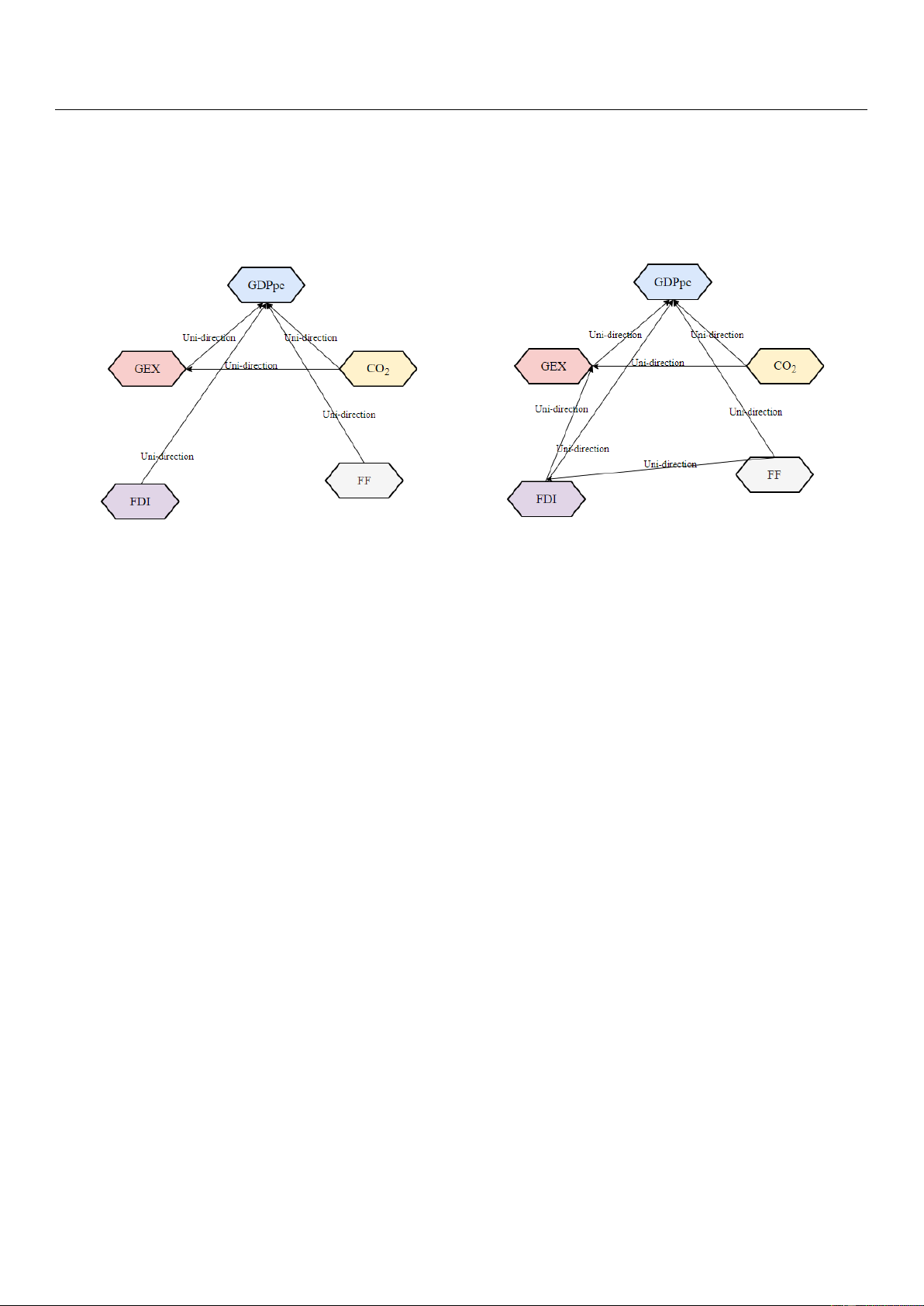
The heterogeneous Granger causalities are evident in the short run. The panel (a) of
Figure 7 shows unidirectional causalities running from GEX, CO2, FDI and FF to GDPpc,
and from CO2 to GEX, in Northern republics. In summary, these causalities imply that GEX
and FF deployment can serve as a catalyst for regional FDI-fueled sustained GDPpc growth.
Nevertheless, policymakers’ biggest obstacle is finding the ideal balance between GEX and
CO2 emissions [88] vv. However, panel (b) of Figure 7 shows unidirectional causalities lOMoAR cPSD| 36066900
Int. J. Environ. Res. Public Health 2022, 19, 10629 18 of 23
running from GEX, CO2, FF and FDI to GDPpc, from GEX to CO2, from FF to FDI, and
from FDI to GEX in Southern Africa. In general, these causalities suggest that the region’s
GDPpc emanates from GEX, FDI, and FF. CO2 should not be overlooked as FDI and FF
increase in the region to improve the growth rate. Again, obtaining a balance between GEX
and CO2 is equally important to the growth of these republics. (a) (b)
Figure 7. The direction of causality. (a) shows unidirectional causalities running from GEX, CO2, FDI
and FF to GDPpc, and from CO2 to GEX, in Northern republics; (b) shows unidirectional causalities
running from GEX, CO2, FF and FDI to GDPpc, from GEX to CO2, from FF to FDI, and from FDI to GEX in Southern Africa. 5. Conclusions
In recent years, there has been a focus on enacting expansionary macroeconomic
policies to mitigate the negative consequences of economic crises. During these years,
GEX in many nations has expanded dramatically, influencing economic performance and
other welfare metrics. Although improving EQ is not a primary aim of fiscal policy, owing
to a lack of public approval, it is vital to analyze the implications of these policies on
the effectiveness of environmental legislation and their possible influence on the level of
pollution. In this regard, this research empirically examines the relationship between EG
and GEX on EQ by evaluating the channels that support the relationship. We investigate
the supposition that EG and EQ improve the mitigating impact of GEX on air pollution
in NASA regions in particular. Using PVAR and quantile regression, data from a panel of
nations from 2000 to 2016 were used to estimate the drivers of LNGDPpc, LNGEX, LNCO2,
LNFF, and LNFDI. The following are the findings of this investigation:
The quantile findings in the North republics show that GEX had a significant posi-
tive effect at all levels of quantiles. However, the marginal effect increases by 1% from
lower to higher quantile. In the South, GEX significantly impacted EQ negatively. The
other determinants (FF, and FDI) of EQ in the South were reported to have no impact on the environment.
In addition, according to the PVAR through the GMM style in North Africa, economic
growth is positive and significant, while the parameter for CO2 is insignificant and negative.
Meaning that the economies of these countries expand with CO2, thus declining EQ, and in
Southern Africa, economic growth is positive and significant while the parameter for CO2
is significant and negative. This implies that as these countries’ economies expand with CO2 emissions, improving EQ.
Moreover, the IRA in North Africa reports that other determinants explain LNGDPpc
by 17%, 17%, 39%, 19.7, and 8.3% for the future variations due to shocks in LNGEX, LNCO2
LNFF, and LNFDI. Moreover, 5.1%, 38.8%, 46.3%, 8.6%, and 1% of future fluctuation in
LNGEX are due to shocks in LNGDPpc, LNFF, LNFDI. In the South, the results show that lOMoAR cPSD| 36066900
Int. J. Environ. Res. Public Health 2022, 19, 10629 19 of 23
66.5%, 5.4%, 21.2%, 0.2%, and 6.7% of future fluctuations in LNGDPpc are due to shocks in LNCO2 LNFF LNGEX, LNFDI.
Lastly, in the granger causality report In North Africa, there is uni-directional cau-
sation running from LNGEX → LNGDPpc, LNCO2 → LNGDPpc, LNFDI → LNGDPpc,
LNCO2 → LNGEX, LNFF → LNGEX, and LNFDI → LNGEX, the granger outcomes sup-
port studies of [24,83] who discovered a one-way relationship between EG, CO2, and FDI.
Similarly, in South republics, unidirectional causation runs from LNGEX → LNCGDPpc,
LNFF → GDPpc, LNFDI → LNGDPpc, LNCO2 → LNGEX, and LNFDI → LNGEX.
5.1. Policy Implication
This study provides confidence to macroeconomic policymakers in NASA republics
that increasing fiscal spending is not harmful to EQ and may significantly relieve air
pollution, particularly in industrialized nations. As a result, fiscal expenditure might be
helpful in extra efforts to reduce air pollution, making them readily and less expensive.
The impact of GEX on EQ in developing countries can be bolstered by reducing policy
flaws such as the protection of industry and energy subsidies and enforcing property rights
over natural resources, which can help internalize environmental outlays the sources of
pollution [89]. Furthermore, policymakers in sub-regional economies in NASA should
stimulate GEX by encouraging green technologies. Thus, policymakers should focus on
GEX to stimulate economic growth and improve the environment (especially the regional
blocs including ECOWAS, CEMAC, EAC, and SADC). The governments in the various
economic syndicates should develop regional policies and incentives to help businesses
adapt to environmentally sustainable production processes, which will help ease the
government’s pressures to improve EQ.
Again, various additional elements that may impact EQ should be addressed when
formulating fiscal policies, such as the composition of GEX and the cumulative effect of
each policy on economic development and government debt sustainability. Finally, it is
critical to construct NASA areas’ sub-regional and macroeconomic policies so that EQ is
improved. Increasing EQ in the nations studied would require changing the composition
of GEX rather than the size. As a result, policymakers should raise the proportion of EX in
GEX. Expanding public-goods spending and replacing private-goods spending, for exam-
ple, might boost EQ by reducing reliance on natural capital, such as energy consumption.
Transferring funds to investments in R&D that promote eco-friendly technologies, such
as the utilization of renewable energy sources, will significantly reduce the number of
pollution-spreading technologies with negative environmental consequences while enhanc-
ing EQ should be considered by governments of NASA regions. The recent COVID-19
pandemic has opened most countries up to newer governmental policies which are geared
toward self-reliant and cleaner technologies which enhance EQ. Future research could look
into using other environmental indicators to investigate the topic.
5.2. Limitation of the Study
Two significant limitations were faced in this study and need attention for future
studies. First, the study period was restricted to 2000–2016 due to data limitations for
the variables and could not include other economic indicators from the selected regions,
which was far shorter than what researchers originally anticipated. When these data are
completely made accessible, researchers advise that future research should take longer
study periods into account. Additionally, because NASA republics differ in terms of their
geographic location, culture, political system, and economic structure, the findings of
this study cannot be extrapolated to other African nations or the entire world. Therefore,
extrapolating data that solely apply to NASA republics to other countries might result in
false conclusions. Despite the aforementioned restrictions, the study’s objectives were met. lOMoAR cPSD| 36066900
Int. J. Environ. Res. Public Health 2022, 19, 10629 20 of 23
Author Contributions: Y.K. supervised the study; M.D. conceptualized and wrote the final manuscript;
E.K.M. analyzed the data and drafted the original manuscript; A.H.N. aided in analysis and discus-
sions; F.A.-T. contributed to the editing and revising of the paper. All authors have read and agreed
to the published version of the manuscript.
Funding: This study was funded by the Nature Fund 2020 (Project Approval Number: 71973054).
Institutional Review Board Statement: Not applicable.
Informed Consent Statement: Not applicable.
Data Availability Statement: World Bank Group. (2020). World Development Indicators 2020,
Washington DC: World Bank. [Dataset for GDP, FDI]. https://datacatalog.worldbank.org/dataset/
world-development-indicators (accessed on 23 October 2021).
Conflicts of Interest: The authors declare no conflict of interest. Abbreviation EX Environmental expenditures EG Economic growth EQ Environmental quality GEX
Government finance expenditure GDPpc GDP per capita NASA
Northern Africa and Southern Africa republics PQR Panel quantile regression PVAR Panel vector autoregressive GMM Generalized method of moment CO2 Carbon dioxide emission FDI Foreign direct investment FF Fossil fuel WWII World War II GHG Greenhouse gases UNFCC
United Nations Framework Convention on Climate Change MENA Middle East/North Africa References 1.
Mesjasz-Lech, A. Environmental Protection Expenditures and Effects of Environmental Governance of Sustainable Development in
Manufacture Enterprise. Available online: https://ideas.repec.org/h/pkk/meb017/244-257.html (accessed on 12 November 2021). 2.
Ssali, M.W.; Du, J.; Mensah, I.A.; Hongo, D.O. Investigating the nexus among environmental pollution, economic growth, energy
use, and foreign direct investment in 6 selected sub-Saharan African countries. Environ. Sci. Pollut. Res. 2019, 26, 11245–11260. [CrossRef] [PubMed] 3.
Asongu, S.A.; Agboola, M.O.; Alola, A.A.; Bekun, F.V. The criticality of growth, urbanization, electricity and fossil fuel consump-
tion to environment sustainability in Africa. Sci. Total Environ. 2020, 712, 136376. [CrossRef] [PubMed] 4.
Is¸ik, C.; Kasımatı, E.; Ongan, S. Analyzing the causalities between economic growth, financial development, international trade,
tourism expenditure and/on the CO2 emissions in Greece. Energy Sources Part B Econ. Plan. Policy 2017, 12, 665–673. [CrossRef] 5.
Zuo, S.; Zhu, M.; Xu, Z.; Oláh, J.; Lakner, Z. The Dynamic Impact of Natural Resource Rents, Financial Development, and
Technological Innovations on Environmental Quality: Empirical Evidence from BRI Economies. Int. J. Environ. Res. Public Health
2021, 19, 130. [CrossRef] [PubMed] 6.
Krajewski, P. The Impact of Public Environmental Protection Expenditure on Economic Growth. Probl. Ekorozw. Probl. Sustain.
Dev. 2016, 11, 99–104. Available online: https://ssrn.com/abstract=2884612 (accessed on 12 November 2021). 7.
Zafar, M.W.; Shahbaz, M.; Hou, F.; Sinha, A. From nonrenewable to renewable energy and its impact on economic growth: The
role of research & development expenditures in Asia-Pacific Economic Cooperation countries. J. Clean. Prod. 2019, 212, 1166–1178. [CrossRef] 8.
European Environmental Agency. “No Title,” Environmental Protection Expenditure. 2016. Available online: http://ec.europa.
eu/environment/action-programme/ (accessed on 11 November 2021). 9.
Ibrahim, M.D.; Alola, A.A.; Cunha Ferreira, D. A two-stage data envelopment analysis of efficiency of social-ecological systems:
Inference from the sub-Saharan African countries. Ecol. Indic. 2021, 123, 107381. [CrossRef]
10. He, L.; Wu, M.; Wang, D.; Zhong, Z. A study of the influence of regional environmental expenditure on air quality in China: T he
effectiveness of environmental policy. Environ. Sci. Pollut. Res. 2018, 25, 7454–7468. [CrossRef] lOMoAR cPSD| 36066900
Int. J. Environ. Res. Public Health 2022, 19, 10629 21 of 23
11. Gholipour, H.F.; Farzanegan, M.R. Institutions and the effectiveness of expenditures on environmental protection: Evidence from
Middle Eastern countries. Const. Political Econ. 2018, 29, 20–39. [CrossRef]
12. UN. The Declaration of the UNs Conference on the Human Environment. 1972. Available online: https://legal.un.org/avl/ha/
dunche/dunche.html (accessed on 23 November 2021).
13. UNFCC. Uniting the World to Tackle Climate Change: COP26 and the Commitments of European Standards. 2021. Available online:
https://www.cencenelec.eu/media/Policy%20Opinions/cen-cenelec_position_paper_cop26.pdf (accessed on 23 November 2021).
14. Furuoka, F. Renewable electricity consumption and economic development: New findings from the Baltic countries. Renew.
Sustain. Energy Rev. 2017, 71, 450–463. [CrossRef]
15. Kim, M.H.; Adilov, N. The lesser of two evils: An empirical investigation of foreign direct investment-pollution tradeoff. Appl.
Econ. 2012, 44, 2597–2606. [CrossRef]
16. Zhao, W.; Xu, Y. Public Expenditure and Green Total Factor Productivity: Evidence from Chinese Prefecture-Level Cities. Int. J.
Environ. Res. Public Health 2022, 19, 5755. [CrossRef] [PubMed]
17. Fan, W.; Li, L.; Wang, F.; Li, D. Driving factors of CO2 emission inequality in China: The role of government expenditure. China
Econ. Rev. 2020, 64, 101545. [CrossRef]
18. Halkos, G.E.; Paizanos, E.A. The channels of the effect of government expenditure on the environment: Evidence using dynamic
panel data. J. Environ. Plan. Manag. 2017, 60, 135–157. [CrossRef]
19. Fincke, B.; Greiner, A. Public Debt and Economic Growth in Emerging Market Economies. S. Afr. J. Econ. 2015, 83, 357–370. [CrossRef]
20. Pyerina-Carmen, G.; Cezar, B.; Eftalea, C.; Ana, E.; Angela, D.; Emilia, V. Insulation materials for buildings—A successful research
and development collaboration for the Romanian wool fibres manufacturing. Ind. Text. 2018, 69, 419–421. [CrossRef]
21. Barra, C.; Zotti, R. Investigating the non-linearity between national income and environmental pollution: International evidence
of Kuznets curve. Environ. Econ. Policy Stud. 2018, 20, 179–210. [CrossRef]
22. Zhu, H.; Xia, H.; Guo, Y.; Peng, C. The heterogeneous effects of urbanization and income inequality on CO2 emissions in BRICS
economies: Evidence from panel quantile regression. Environ. Sci. Pollut. Res. 2018, 25, 17176–17193. [CrossRef]
23. Xie, J.Y.; Suh, D.H.; Joo, S.-K. A Dynamic Analysis of Air Pollution: Implications of Economic Growth and Renewable Energy
Consumption. Int. J. Environ. Res. Public Health 2021, 18, 9906. [CrossRef]
24. Odhiambo, N.M. CO2 emissions and economic growth in sub-Saharan African countries: A panel data analysis. Int. Area Stud.
Rev. 2017, 20, 264–272. [CrossRef]
25. Espoir, D.K.; Sunge, R.; Bannor, F. CO2 emissions and economic development in Africa: Evidence from a dynamic spatial panel
model. J. Environ. Manag. 2021, 300, 113617. [CrossRef]
26. Musah, M.; Kong, Y.; Mensah, I.A.; Antwi, S.K.; Donkor, M. The link between carbon emissions, renewable energy consumption,
and economic growth: A heterogeneous panel evidence from West Africa. Environ. Sci. Pollut. Res. 2020, 27, 28867–28889. [CrossRef]
27. Mensah, I.A.; Sun, M.; Gao, C.; Omari-Sasu, A.Y.; Zhu, D.; Ampimah, B.C.; Quarcoo, A. Analysis on the nexus of economic
growth, fossil fuel energy consumption, CO2 emissions and oil price in Africa based on a PMG panel ARDL approach. J. Clean.
Prod. 2019, 228, 161–174. [CrossRef]
28. Orubu, O.C.; Omotor, G.D. Environmental quality and economic growth: Searching for environmental Kuznets curves for air and
water pollutants in Africa. Energy Policy 2011, 39, 4178–4188. [CrossRef]
29. Barreto, H. Omitted Variable Bias. In Introductory Econometrics: Using Monte Carlo Simulation with Microsoft Excel; Cambridge
University Press: Cambridge, UK, 2006.
30. Clarke, K.A. The Phantom Menace: Omitted Variable Bias in Econometric Research. Confl. Manag. Peace Sci. 2005, 22, 341–352. [CrossRef]
31. Baz, K.; Cheng, J.; Xu, D.; Abbas, K.; Ali, I.; Ali, H.; Fang, C. Asymmetric impact of fossil fuel and renewable energy consu mption
on economic growth: A nonlinear technique. Energy 2021, 226, 120357. [CrossRef]
32. Hadj, T.B. Nonlinear impact of biomass energy consumption on ecological footprint in a fossil fuel –dependent economy. Environ.
Sci. Pollut. Res. 2021, 28, 69329–69342. [CrossRef]
33. Ekwueme, D.C.; Zoaka, J.D.; Alola, A.A. Carbon emission effect of renewable energy utilization, fiscal development, and forei gn
direct investment in South Africa. Environ. Sci. Pollut. Res. 2021, 28, 41821–41833. [CrossRef]
34. Vo, X.V.; Zaman, K. Relationship between energy demand, financial development, and carbon emissions in a panel of 101
countries: “go the extra mile” for sustainable development. Environ. Sci. Pollut. Res. 2020, 27, 23356–23363. [CrossRef]
35. Naz, S.; Sultan, R.; Zaman, K.; Aldakhil, A.M.; Nassani, A.A.; Abro, M.M.Q. Moderating and mediating role of renewable energy
consumption, FDI inflows, and economic growth on carbon dioxide emissions: Evidence from robust least square estimator.
Environ. Sci. Pollut. Res. 2019, 26, 2806–2819. [CrossRef]
36. Chenran, X.; Limao, W.; Chengjia, Y.; Qiushi, Q.; Ning, X. Measuring the Effect of Foreign Direct Investment on CO 2 Emissions in
Laos. J. Resour. Ecol. 2019, 10, 685. [CrossRef]
37. Aluko, O.A.; Ibrahim, M. Institutions and the financial development–economic growth nexus in sub-Saharan Africa. Econ. Notes
2020, 49, e12163. [CrossRef] lOMoAR cPSD| 36066900
Int. J. Environ. Res. Public Health 2022, 19, 10629 22 of 23
38. Musah, M.; Kong, Y.; Mensah, I.A.; Antwi, S.K.; Osei, A.A.; Donkor, M. Modelling the connection between energy consumption
and carbon emissions in North Africa: Evidence from panel models robust to cross-sectional dependence and slope heterogeneity.
Environ. Dev. Sustain. 2021, 23, 15225–15239. [CrossRef]
39. Al-Moulani, A.; Alexiou, C. Banking sector depth and economic growth nexus: A comparative study between the natural
resource-based and the rest of the world’s economies. Int. Rev. Appl. Econ. 2017, 31, 625–650. [CrossRef]
40. Bernauer, T.; Koubi, V. States as Providers of Public Goods: How Does Government Size Affect Environmental Quality? SSRN
Electron. J. 2006. [CrossRef]
41. López, R.; Galinato, G.I.; Islam, A. Fiscal spending and the environment: Theory and empirics. J. Environ. Econ. Manag.
2011, 62, 180–198. [CrossRef]
42. Lin, Q.; Chen, G.; Du, W.; Niu, H. Spillover effect of environmental investment: Evidence from panel data at provincial level in
China. Front. Environ. Sci. Eng. 2012, 6, 412–420. [CrossRef]
43. Halkos, G.E.; Paizanos, E.A. The effect of government expenditure on the environment:An empirical investigation. Ecol. Econ.
2013, 91, 48–56. [CrossRef]
44. López, R.; Palacios, A. Why has Europe Become Environmentally Cleaner? Decomposing the Roles of Fiscal, Trade and
Environmental Policies. Environ. Resour. Econ. 2014, 58, 91–108. [CrossRef]
45. Islam, A.M.; López, R.E. Government Spending and Air Pollution in the US. Int. Rev. Environ. Resour. Econ. 2015, 8, 139–189. [CrossRef]
46. Galinato, G.I.; Galinato, S.P. The effects of government spending on deforestation due to agricultural land expansion and CO2
related emissions. Ecol. Econ. 2016, 122, 43–53. [CrossRef]
47. Raworth, K. Doughnut Economics: Seven Ways to Think Like a 21st-Century Economist; Random House Business: New York, NY,
USA, 2017; Available online: https://www.amazon.com/Doughnut-Economics-Seven-21st-Century-Economist/dp/1603586741
(accessed on 26 December 2021).
48. Anwar, A.; Sinha, A.; Sharif, A.; Siddique, M.; Irshad, S.; Anwar, W.; Malik, S. The nexus between urbanization, renewable
energy consumption, financial development, and CO2 emissions: Evidence from selected Asian countries. Environ. Dev. Sustain.
2022, 24, 6556–6576. [CrossRef]
49. Sunkanmi, O.; Nurudeen, A.; Usman, A. Government Expenditure and Economic Growth in Nigeria, 1970–2008: A Disaggregated
Analysis. Bus. Econ. J. 2010, 2010, BEJ-4. Available online: http://astonjournals.com/bej (accessed on 13 December 2021).
50. Haug, A.A.; Ucal, M. The role of trade and FDI for CO2 emissions in Turkey: Nonlinear relationships. Energy Econ.
2019, 81, 297–307. [CrossRef]
51. Rehman, A.; Ma, H.; Ahmad, M.; Ozturk, I.; Is¸ık, C. An asymmetrical analysis to explore the dynamic impacts of CO2 emission to
renewable energy, expenditures, foreign direct investment, and trade in Pakistan. Environ. Sci. Pollut. Res. 2021, 28, 53520–53532. [CrossRef] [PubMed]
52. Is¸ık, C.; Ongan, S.; Özdemir, D. Testing the EKC hypothesis for ten US states: An application of heterogeneous panel estimation
method. Environ. Sci. Pollut. Res. 2019, 26, 10846–10853. [CrossRef]
53. Isik, C.; Ongan, S.; Özdemir, D. The economic growth/development and environmental degradation: Evidence from the US
state-level EKC hypothesis. Environ. Sci. Pollut. Res. 2019, 26, 30772–30781. [CrossRef]
54. Kivyiro, P.; Arminen, H. Carbon dioxide emissions, energy consumption, economic growth, and foreign direct investment:
Causality analysis for Sub-Saharan Africa. Energy 2014, 74, 595–606. [CrossRef]
55. Hamilton, T.G.A.; Kelly, S. Low carbon energy scenarios for sub-Saharan Africa: An input-output analysis on the effects of
universal energy access and economic growth. Energy Policy 2017, 105, 303–319. [CrossRef]
56. Keynes, J.M. Las Posibilidades Económicas de Nuestros Nietos: Una Lectura de Keynes por Joaquín Estefanía; Taurus: Madrid, Spain, 2015; pp. 20–255.
57. Bergh, A.; Karlsson, M. Government size and growth: Accounting for economic freedom and globalization. Public Choice
2010, 142, 195–213. [CrossRef]
58. Zimcˇík, P. Economic Growth and Budget Constraints: EU Countries Panel Data Analysis. Rev. Econ. Perspect. 2016, 16, 87–101. [CrossRef]
59. Jiranyakul, K. The Relation between Government Expenditures and Economic Growth in Thailand. SSRN Electron. J. 2013. [CrossRef]
60. Tatahi, M.; Cetin, E.I.; Cetin, M.K. The Cause of Higher Economic Growth: Assessing the Long-Term and Short-Term Relationships
between Economic Growth and Government Expenditure. Macroecon. Dyn. 2016, 20, 229–250. [CrossRef]
61. Chandio, A.A.; Jiang, Y.; Rehman, A.; Jingdong, L. Impact of Government Expenditure on Agricultural Sector and Economic
Growth in Pakistan. Int. J. Adv. Biotechnol. Res. 2016, 7, 1046–1053.
62. Khac Lich, H.; Cam Tu, D. The Optimal Public Expenditure in Developing Countries. VNU J. Sci. Econ. Bus. 2019, 35. [CrossRef]
63. Is¸ık, C.; Ongan, S.; Bulut, U.; Karakaya, S.; Irfan, M.; Alvarado, R.; Ahmad, M.; Rehman, A. Reinvestigating the Environmental
Kuznets Curve (EKC) hypothesis by a composite model constructed on the Armey curve hypothesis with government spending
for the US States. Environ. Sci. Pollut. Res. 2020, 29, 16472–16483. [CrossRef]
64. Manu, E.K.; Xuezhou, W.; Paintsil, I.O.; Gyedu, S.; Ntarmah, A.H. Financial development and economic growth nexus in Africa.
Bus. Strateg. Dev. 2020, 3, 506–521. [CrossRef] lOMoAR cPSD| 36066900
Int. J. Environ. Res. Public Health 2022, 19, 10629 23 of 23
65. World Bank. Environment in Mena, Sector Brief. World Bank Group. 2008. Available online: http://web.worldbank.org/archive/
website01418/WEB/IMAGES/ENVIR-12.PDF (accessed on 17 December 2021).
66. Croitoru, L.; Sarraf, M. The Cost of Environmental Degradation: Case Studies from the Middle East and North Africa. 2010.
Available online: https://openknowledge.worldbank.org/handle/10986/2499 (accessed on 29 November 2021).
67. Yaduma, N.; Kortelainen, M.; Wossink, A. The environmental Kuznets curve at different levels of economic development: A
counterfactual quantile regression analysis for CO2 emissions. J. Environ. Econ. Policy 2015, 4, 278–303. [CrossRef]
68. World Bank Group. World Development Indicators; World Bank Group: Washington, DC, USA, 2020; Available online: https:
//datatopics.worldbank.org/world-development-indicators/ (accessed on 29 November 2021).
69. Ahmad, M.; Zhao, Z.-Y.; Irfan, M.; Mukeshimana, M.C. Empirics on influencing mechanisms among energy, finance, trade,
environment, and economic growth: A heterogeneous dynamic panel data analysis of China. Environ. Sci. Pollut. Res.
2019, 26, 14148–14170. [CrossRef]
70. Bekhet, H.A.; Matar, A.; Yasmin, T. CO2 emissions, energy consumption, economic growth, and financial development in GCC
countries: Dynamic simultaneous equation models. Renew. Sustain. Energy Rev. 2017, 70, 117–132. [CrossRef]
71. Rice, W.R. A Consensus Combined P-Value Test and the Family-Wide Significance of Component Tests. Biometrics 1990, 46, 303. [CrossRef]
72. Qian, X.; Chen, G.; Kattel, B.; Lee, S.; Yang, Y. Factorial analysis of vertical ground reaction force and required coefficient of
friction for safety of stair ascent and descent. Int. J. Ind. Oper. Res. 2018, 1, 002. [CrossRef]
73. Balsalobre-Lorente, D.; Shahbaz, M.; Roubaud, D.; Farhani, S. How economic growth, renewable electricity and natural resources
contribute to CO2 emissions? Energy Policy 2015, 113, 356–367. [CrossRef]
74. Komen, M.H.; Gerking, S.; Folmer, H. Income and environmental R&D: Empirical evidence from OECD countries. Environ. Dev.
Econ. 1997, 2, 505–515. [CrossRef]
75. Mohammed Saud, M.A.; Guo, P.; Haq, I.U.; Pan, G.; Khan, A. Do government expenditure and financial development impede
environmental degradation in Venezuela? PLoS ONE 2019, 14, e0210255. [CrossRef]
76. Machado, J.A.F.; Santos Silva, J.M.C. Quantiles via moments. J. Econom. 2019, 213, 145–173. [CrossRef]
77. Sherwood, B. Variable selection for additive partial linear quantile regression with missing covariates. J. Multivar. Anal.
2016, 152, 206–223. [CrossRef]
78. Zhu, H.; Duan, L.; Guo, Y.; Yu, K. The effects of FDI, economic growth and energy consumption on carbon emissions in ASEAN-5:
Evidence from panel quantile regression. Econ. Model. 2016, 58, 237–248. [CrossRef]
79. Xuezhou, W.; Manu, E.K.; Akowuah, I.N. Financial development and environmental quality: The role of economic growth among
the regional economies of Sub-Saharan Africa. Environ. Sci. Pollut. Res. 2021, 29, 23069–23093. [CrossRef]
80. Arcand, J.-L.; Berkes, E.; Panizza, U. Too Much Finance; IMF: Washington, DC, USA, 2012.
81. Andrews, D.W.K.; Lu, B. Consistent model and moment selection procedures for GMM estimation with application to dynamic
panel data models. J. Econom. 2001, 101, 123–164. [CrossRef]
82. Love, I.; Zicchino, L. Financial development and dynamic investment behavior: Evidence from panel VAR. Econ. Financ.
2006, 46, 190–210. [CrossRef]
83. Shoaib, H.M.; Rafique, M.Z.; Nadeem, A.M.; Huang, S. Impact of financial development on CO2 emissions: A comparative
analysis of developing countries (D8) and developed countries (G8). Environ. Sci. Pollut. Res. 2020, 27, 12461–12475. [CrossRef] [PubMed]
84. Muhammad, B.; Khan, S. Effect of bilateral FDI, energy consumption, CO2 emission and capital on economic growth of Asia
countries. Energy Rep. 2019, 5, 1305–1315. [CrossRef]
85. Asumadu-Sarkodie, S.; Owusu, P.A. Carbon dioxide emissions, GDP, energy use, and population growth: A multivariate and
causality analysis for Ghana, 1971–2013. Environ. Sci. Pollut. Res. 2016, 23, 13508–13520. [CrossRef]
86. Granger, C.W.J. Causality, cointegration, and control. J. Econ. Dyn. Control 1988, 12, 551–559. [CrossRef]
87. Gani, A. Fossil fuel energy and environmental performance in an extended STIRPAT model. J. Clean. Prod. 2021, 297, 126526. [CrossRef]
88. Manu, E.K.G.S.C.; Asante, D. Regional heterogeneities in the absorptive capacity of renewable energy deployment in Africa.
Renew. Energy 2022, 193, 554–564. [CrossRef]
89. Panayotou, T. Green Markets: The Economics of Sustainable Development. 1993. Available online: https://www.cabdirect.org/
cabdirect/abstract/19946797014 (accessed on 30 December 2021).
Tài liệu liên quan:
-
Chapter 2 Principles of Microeconomic | Bài giảng kinh tế học vi mô
78 39 -

Chapter 6 The Market Structures | Bài giảng kinh tế học vi mô
81 41 -

Tài liệu sưu tầm, Bài tập chương 2. Kinh tế vi mô
58 29 -

Tài liệu sưu tầm, Bài tập chương 1. Kinh tế vi mô
58 29 -

Giáo Trình Kinh Tế Vi Mô - Bản PDF Chất Lượng Cao
118 59