EOQ Analysis: Demand, Costs, and Inventory Management Strategies | Thực tập cơ bản | Trường Đại học Bách Khoa Hà Nội
5.2Define parameters:D = annual demand (units/year) S = ordering cost per order H = holding (carrying) cost per unit per year . Tài liệu giúp bạn tham khảo, ôn tập và đạt kết quả cao. Mời đọc đón xem!
Môn: Thực tập cơ bản 331 tài liệu
Trường: Đại học Bách Khoa Hà Nội 5.6 K tài liệu
Tác giả:


Preview text:
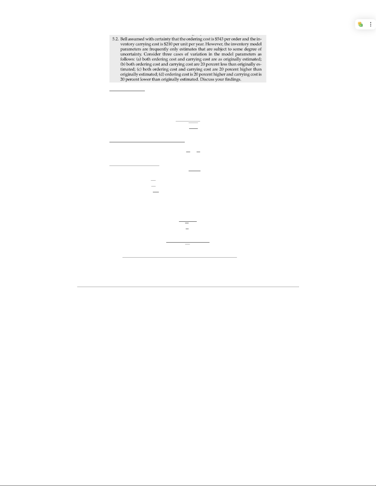
5.2 Define parameters: D = annual demand (units/year) S = ordering cost per order
H = holding (carrying) cost per unit per year √ EOQ formula: Q∗¿ 2DS H QS+Q
Total Cost = Ordering Cost + Holding Cost =D 2H ( ) TC Q √
Minimum total cost at EOQ: TC∗¿ √2DSH Q* depends on S H √ TC* depends on SH
Let a and b be the proportion of the original S and H, respectively √ Then: b× Q∗¿ New EOQ: Q'= a
New minimal total cost: T C'= √ab×TC∗¿ a. Both
ordering cost and carrying cost are as originally estimated
S0 = $543, H0 = $210 are baseline values. Denote the baseline EOQ and TC as Q* and TC* respectively. b. both
ordering cost and carrying cost are 20 percent less than originally estimated S′=0.8S0, H′=0.8H0 Q'= √0.8 0.8×Q∗¿Q∗¿
TC'= √0.8×0.8×TC∗¿0.8TC∗¿
=> Total ordering + holding cost falls by 20% => EOQ remains unchanged
When both costs fall in the same proportion, the optimal order size does not change
(because the ratio S/HS/HS/H stays constant). However, the overall cost of managing
inventory falls proportionally, so the firm spends less on both ordering and carrying. c. Both
ordering cost and carrying cost are 20 percent less than originally estimated S′=1.2S0, H′=1.2H0 Q'= √1.2 1.2×Q∗¿Q∗¿
TC'= √1.2×1.2×TC∗¿1.2TC∗¿
=> Total ordering + holding cost increases by 20% => EOQ remains unchanged
The order policy (lot size) remains unchanged, but the company now spends more due to
higher costs. This shows that EOQ is robust to proportional estimation errors in S and H d. Ordering
cost is 20 percent higher and carrying cost is 20 percent lower than
originally estimated S′=1.2S0, H′=0.8H0 Q'= √1.2 0.8×Q∗¿ √1.5Q∗¿ => EOQ increases ≈ 22.5%
TC'= √1.2×0.8×TC∗¿ √0.96TC∗¿
=> total ordering + holding cost slightly decreases ≈ 2.0%
The higher ordering cost encourages larger, less frequent orders. The lower carrying cost
also makes it cheaper to hold more inventory. Together, these forces increase the EOQ
substantially. Interestingly, the total cost drops slightly, because the decrease in holding
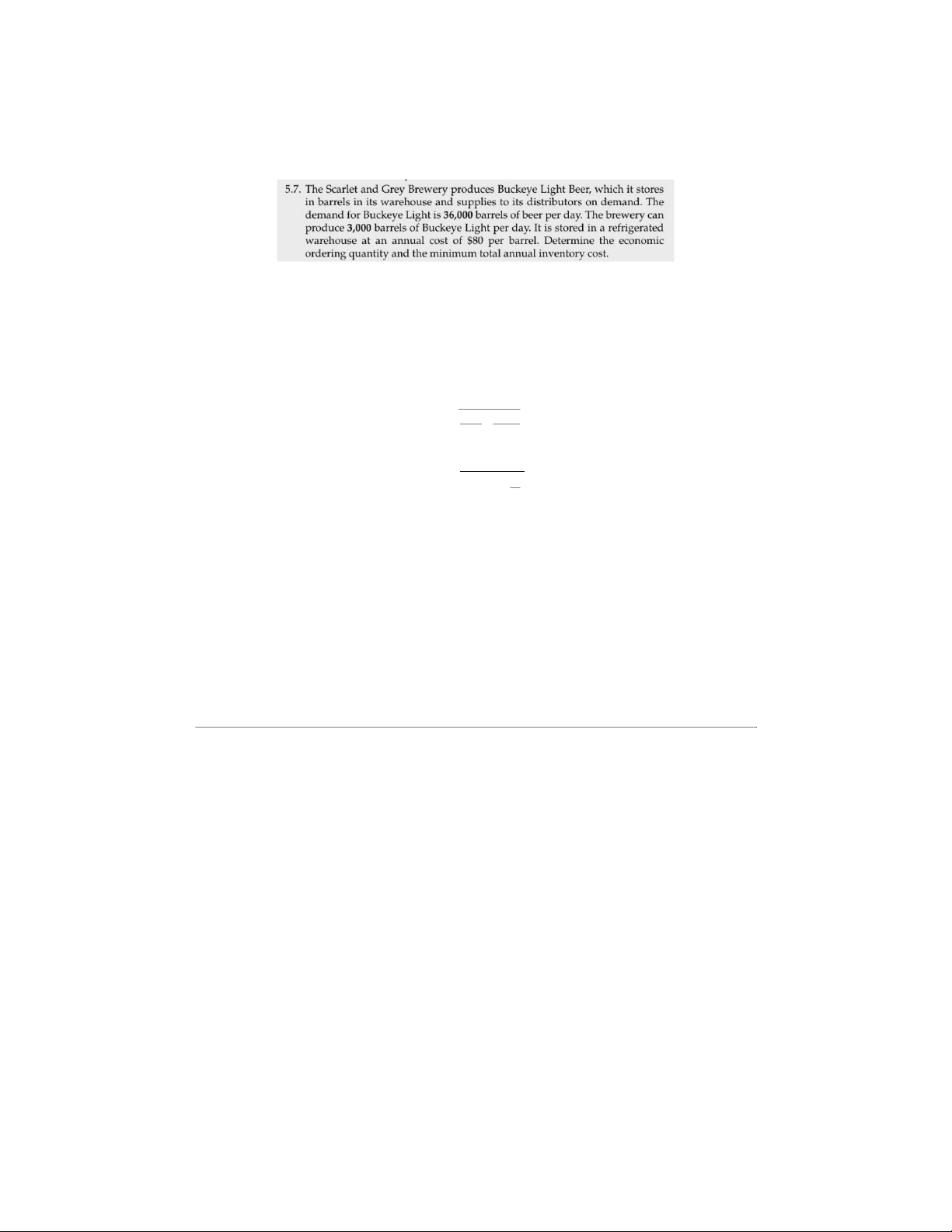
cost outweighs the increase in ordering cost. 5.7 Define parameters: P = annual production D = annual demand H = Holding cost EPQ formulas:
Optimal production lot size per run: Q∗¿ √2DS H×P P−D
Minimal total annual cost: TC∗¿ √2DSH (1−D ) P
Compute constants into formulas:
P = 3,000 barrels/day×365 =1,095,000 barrels/year D = 36,000 barrels/year H = $80 per barrel per year 80×1,095,000
Q∗¿ √2×36,000×S 1,095,000−36,000= √930.5949×S
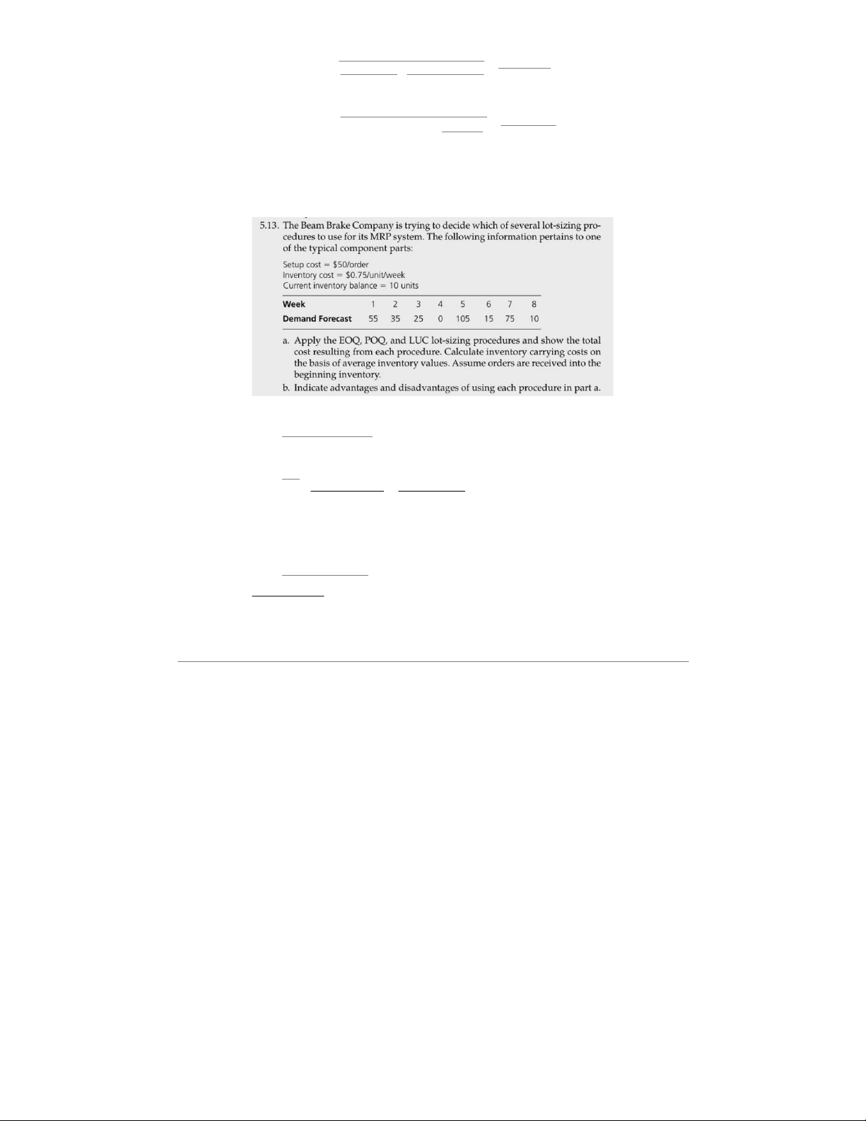
TC∗¿ √2×36,000×80×S× (1−36,000 )= √5,570,630×S 1,095,000 5.13 1) EOQ Procedure Average
demand D week
Dweek = (55+35+25+0+105+15+75+10)/8=40units/week EOQ
Q∗¿ √2×Dweek ×S /H= √2×40×50 / 0.75≈73.03 → Q = 73 (rounded)
The Order quantity of week 3, 4, 8 is 0 since beginning inventory before demand ≥ demand
of the current week, then no new order is placed.
Ex: Week 3: 66¿25 → Order quantity of week 3 = 0 Beginning
inventory For the first week:
Beg inventory = current inventory + EOQ
Ex: Week 1: Beg inventory = 73 + 10 = 83 For week n:
Beg inventory = End inventory of week n-1 + EOQ Ending
inventory
End inventory = Beg inventory – Demand
Ex: Week 1: End inventory = 83 – 55 = 28 Average
inventory for the week
Avg inventory = (Beg inventory + End inventory)/2
Ex: Week 1: Avg inventory = (83 + 28)/2 = 55.5 Holding
cost
Holding cost = Inventory cost per unit per week x Average inventory per week
Ex: Week 1: Holding cost = $0.75 x 55.5 = 41.625
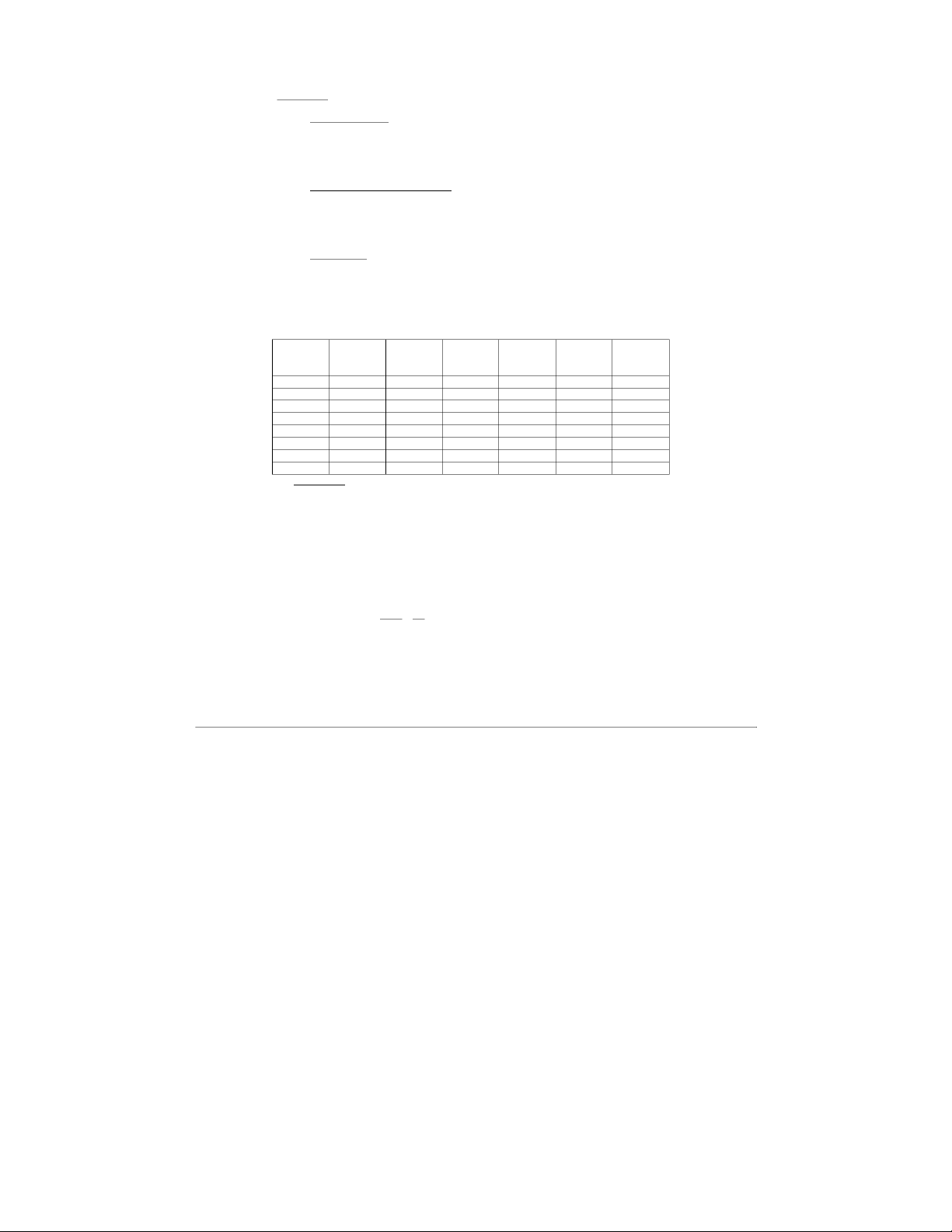
EOQ week-by-week schedule (orders received at beginning of week): Week (n) Demand Order Beg End Avg Holding quantity Inventory inventory inventory cost (Q*) 1 55 73 83 28 55.5 41.625 2 35 73 101 66 83.5 62.62 3 25 0 66 41 53.5 40.12 4 0 0 41 41 41.0 30.75 5 105 73 114 9 61.5 46.12 6 15 73 82 67 74.5 55.88 7 75 73 140 65 102.5 76.88 8 10 0 65 55 60.0 45.0 EOQ totals:
Total numbers of orders = 5 → Setup cost = 5 x $50 = $250 8
Holding cost total = ∑ Holdingcost = $399 n=1
Total inventory cost (EOQ) = Setup cost + Holding cost total = $250 + $399 = $649
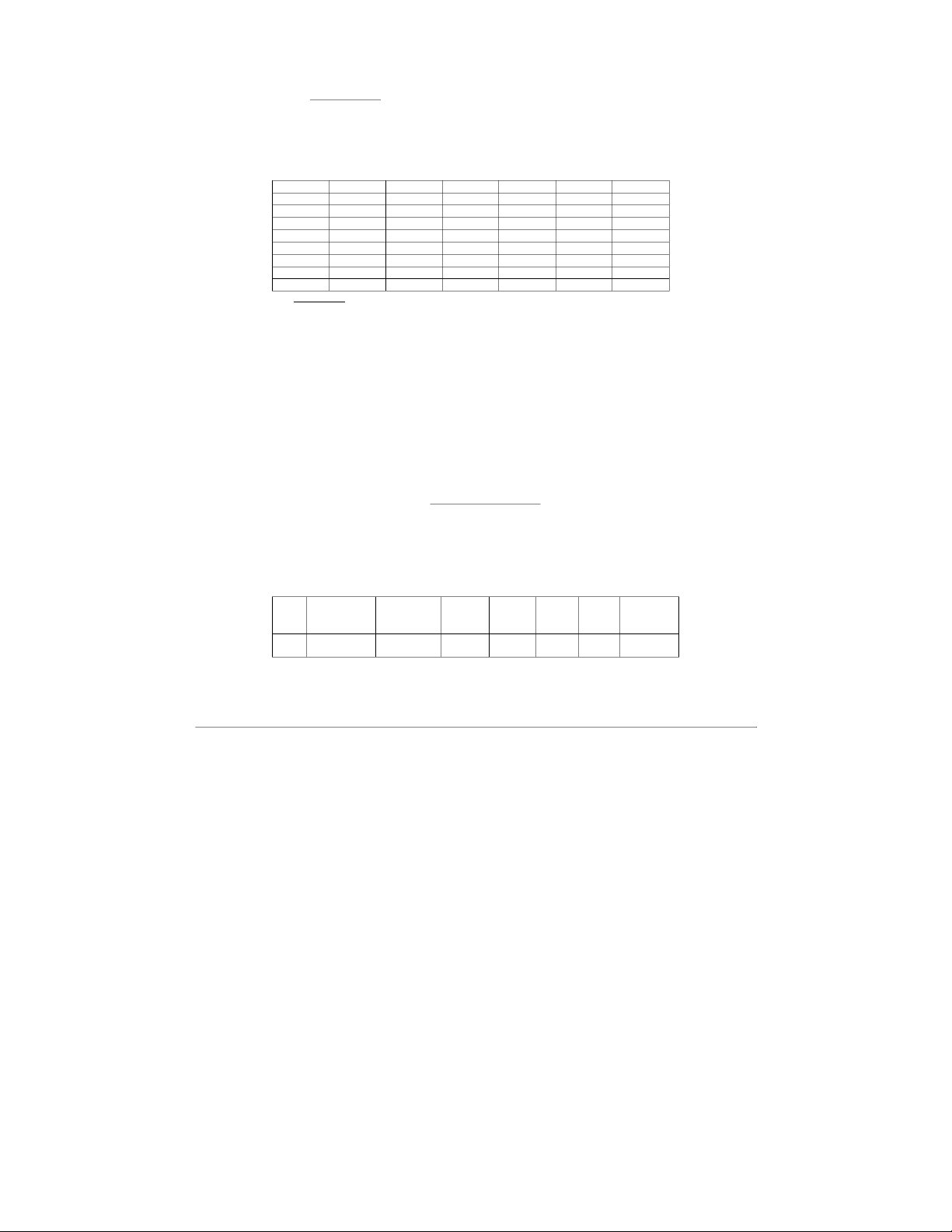
2) POQ Procedure N=Q∗¿ D=73 POQ period chosen
4=1.83weeks=2¿ → Under POQ, every time we order, we
order enough to cover two weeks’ demand Order
quantity:
Order qty = Sum of demand of two weeks
Ex: Week 1: Order qty = 55+35 = 90
The order quantity in week 2, 4, 6, 8 = 0 since we have ordered enough for two weeks. Week Demand Order qty Beg inv End inv Avg inv Hold cost 1 55 90 100 45 72.5 54.38 2 35 0 45 10 27.5 20.62 3 25 25 35 10 22.5 16.88 4 0 0 10 10 10.0 7.5 5 105 120 130 25 77.5 58.12 6 15 0 25 10 17.5 13.12 7 75 85 95 20 57.5 43.12 8 10 0 20 10 15.0 11.25 POQ totals:
Total numbers of orders = 4 → Setup cost = 4 x $50 = $200 Holding cost total = $225
Total inventory cost (POQ) = $200 + $225 = $425
3) LUC (Least Unit Cost) Procedure
The idea of LUC
At a week when inventory is not enough, we must place an order. Instead of always
ordering EOQ (fixed Q) or covering a fixed period (POQ), LUC solve the problem of how
many future weeks this order should cover.
To decide, we try k=1,2, 3,… weeks ahead. For each k, we calculate:
Unit Cost=Setupcost+Holdingcost Totaldemand¿cover¿
Then we choose the k that gives the lowest unit cost
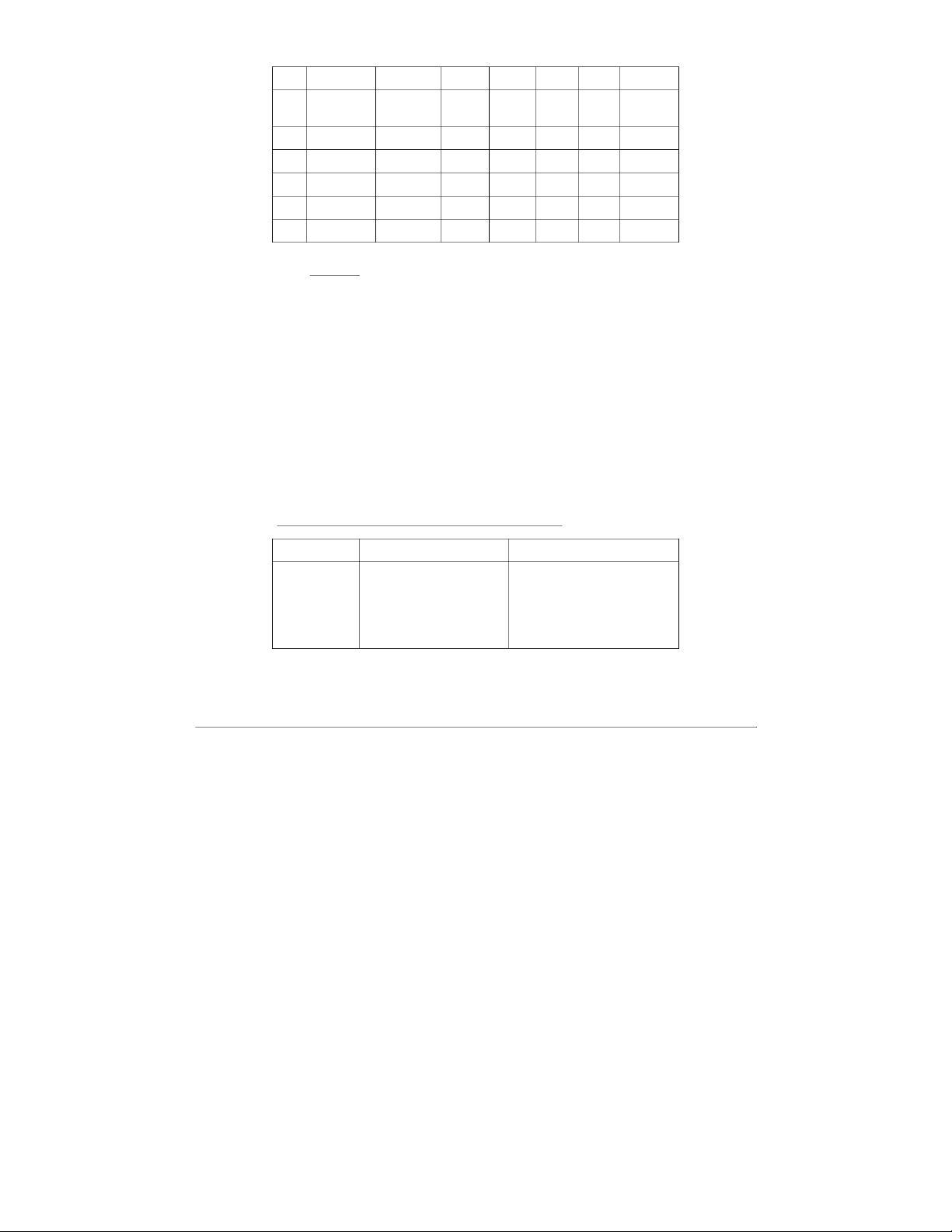
Week-by-week LUC results (orders received at beginning of week): Week Beg inv Order k Demand End Avg Holding placed chosen inv inv ($) 1 10 + 80 = 90 80 k = 2 55 35 62.5 46.875 2 35 0 – 35 0 17.5 13.125 3 0 + 130 = 130 k = 3 25 105 117.5 88.125 130 4 105 0 – 0 105 105.0 78.750 5 105 0 – 105 0 52.5 39.375 6 0 + 90 = 90 90 k = 2 15 75 82.5 61.875 7 75 0 – 75 0 37.5 28.125 8 0 + 10 = 10 10 k = 1 10 0 5.0 3.750 LUC totals:
Number of orders = 4→ Setup cost = 4 * $50 = $200 Holding cost total = $360
Total inventory cost (LUC) = $200 + $360 = $560
4) Summary Comparison Method # Orders Setup Cost Holding Cost Total Cost EOQ 5 $250 $399 $649 POQ 4 $200 $225 $425 LUC 3 $200 $360 $560
→ The optimal method is POQ with period chosen N = 2
b. The advantages and disadvantages of using each procedure Method Advantages Disadvantages
EOQ (Economic - Simple and widely used
- Assumes steady demand → not Order Quantity) formula. realistic with uneven weekly demand. - Balances setup cost and holding cost well when demand
- May cause shortages or excess is stable and constant. stock when demand fluctuates. - Easy to compute and explain
- More frequent orders (higher to managers. setups) → higher cost. POQ (Periodic
- Adjusts EOQ into a time-based - Requires calculation of T* (a little Order Quantity)
cycle (T*), making it practical more complex than EOQ). for uneven demand.
- If demand pattern shifts suddenly, - Groups periods together,
grouping may not align perfectly. reducing average inventory.
- Still based on averages, not per-unit - Fewer stockouts compared to optimization. EOQ.
LUC (Least Unit - Flexible: tests different
- More complex: requires repeated Cost) horizons (k) and chooses the
cost calculations at each decision lowest cost per unit. point. - Adapts well when demand is
- May lead to larger lot sizes → irregular.
higher holding costs (like in our case: $560).
- Helps avoid very small orders.
- Not always optimal globally, it’s a
short-term method, may lead to very high holding costs.
Tài liệu liên quan:
-
Báo cáo Thực Tập Cơ Bản: Linh Kiện và IC Trong Mạch Điện | Thực tập cơ bản | Trường Đại học Bách khoa Hà Nội
41 21 -
Báo cáo Thực Tập Cơ Bản: Thiết Kế Mạch Điện Tử | Thực tập cơ bản | Trường Đại học Bách khoa Hà Nội
35 18 -
Báo cáo về Chủ nghĩa Xã hội Khoa học và Vai trò của C. Mác - Ph. Ăngghen | Thực tập cơ bản | Trường Đại học Bách khoa Hà Nội
40 20 -
Báo cáo Thực Tập Cơ Bản: Thiết Kế Mạch Đếm Thuận 0-9 Bằng Altium | Thực tập cơ bản | Trường Đại học Bách khoa Hà Nội
35 18 -
Báo cáo thực tập Mạch khuếch đại âm tần - Điện tử | Thực tập cơ bản | Trường Đại học Bách khoa Hà Nội
38 19