Exploratory Data Analysis| Giáo trình quản trị dữ liệu và trực quan hóa| Trường Đại học Bách Khoa Hà Nội

Summary

What is exploratory data analysis? How did it begin? How and where did it originate? How is it differentiated from other data analysis approaches, such as classical and Bayesian? Is EDA the same as statistical graphics? What role does statistical graphics play in EDA? Is statistical graphics identical to EDA?

Thông tin:
822 trang 3 tháng trước

Bình luận

Vui lòng đăng nhập hoặc đăng ký để gửi bình luận.

Exploratory Data Analysis| Giáo trình quản trị dữ liệu và trực quan hóa| Trường Đại học Bách Khoa Hà Nội

Summary

What is exploratory data analysis? How did it begin? How and where did it originate? How is it differentiated from other data analysis approaches, such as classical and Bayesian? Is EDA the same as statistical graphics? What role does statistical graphics play in EDA? Is statistical graphics identical to EDA?

25 13 lượt tải Tải xuống
1.Exploratory Data Analysis
This chapter presents the assumptions, principles, and techniques necessary to gain
insight into data via EDA--exploratory data analysis.
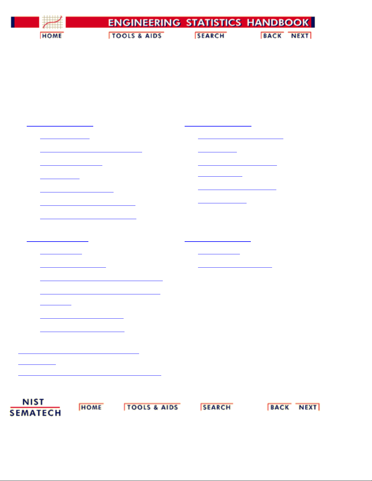
1. EDA Introduction
What is EDA?1.
EDA vs Classical & Bayesian2.
EDA vs Summary3.
EDA Goals4.
The Role of Graphics5.
An EDA/Graphics Example6.
General Problem Categories7.
2. EDA Assumptions
Underlying Assumptions1.
Importance2.
Techniques for Testing
Assumptions
3.
Interpretation of 4-Plot4.
Consequences5.
3. EDA Techniques
Introduction1.
Analysis Questions2.
Graphical Techniques: Alphabetical3.
Graphical Techniques: By Problem
Category
4.
Quantitative Techniques5.
Probability Distributions6.
4. EDA Case Studies
Introduction1.
By Problem Category2.
Detailed Chapter Table of Contents
References
Dataplot Commands for EDA Techniques
1. Exploratory Data Analysis
http://www.itl.nist.gov/div898/handbook/eda/eda.htm [5/1/2006 9:56:13 AM]
1. Exploratory Data Analysis - Detailed Table of
Contents [1.]
This chapter presents the assumptions, principles, and techniques necessary to gain insight into
data via EDA--exploratory data analysis.
EDA Introduction [1.1.]
What is EDA? [1.1.1.]1.
How Does Exploratory Data Analysis differ from Classical Data Analysis? [1.1.2.]
Model [1.1.2.1.]1.
Focus [1.1.2.2.]2.
Techniques [1.1.2.3.]3.
Rigor [1.1.2.4.]4.
Data Treatment [1.1.2.5.]5.
Assumptions [1.1.2.6.]6.
2.
How Does Exploratory Data Analysis Differ from Summary Analysis? [1.1.3.]3.
What are the EDA Goals? [1.1.4.]4.
The Role of Graphics [1.1.5.]5.
An EDA/Graphics Example [1.1.6.]6.
General Problem Categories [1.1.7.]7.
1.
EDA Assumptions [1.2.]
Underlying Assumptions [1.2.1.]1.
Importance [1.2.2.]2.
Techniques for Testing Assumptions [1.2.3.]3.
Interpretation of 4-Plot [1.2.4.]4.
Consequences [1.2.5.]
Consequences of Non-Randomness [1.2.5.1.]1.
Consequences of Non-Fixed Location Parameter [1.2.5.2.]2.
5.
2.
1. Exploratory Data Analysis
http://www.itl.nist.gov/div898/handbook/eda/eda_d.htm (1 of 8) [5/1/2006 9:55:58 AM]
Consequences of Non-Fixed Variation Parameter [1.2.5.3.]3.
Consequences Related to Distributional Assumptions [1.2.5.4.]4.
EDA Techniques [1.3.]
Introduction [1.3.1.]1.
Analysis Questions [1.3.2.]2.
Graphical Techniques: Alphabetic [1.3.3.]
Autocorrelation Plot [1.3.3.1.]
Autocorrelation Plot: Random Data [1.3.3.1.1.]1.
Autocorrelation Plot: Moderate Autocorrelation [1.3.3.1.2.]2.
Autocorrelation Plot: Strong Autocorrelation and Autoregressive
Model [1.3.3.1.3.]
3.
Autocorrelation Plot: Sinusoidal Model [1.3.3.1.4.]4.
1.
Bihistogram [1.3.3.2.]2.
Block Plot [1.3.3.3.]3.
Bootstrap Plot [1.3.3.4.]4.
Box-Cox Linearity Plot [1.3.3.5.]5.
Box-Cox Normality Plot [1.3.3.6.]6.
Box Plot [1.3.3.7.]7.
Complex Demodulation Amplitude Plot [1.3.3.8.]8.
Complex Demodulation Phase Plot [1.3.3.9.]9.
Contour Plot [1.3.3.10.]
DEX Contour Plot [1.3.3.10.1.]1.
10.
DEX Scatter Plot [1.3.3.11.]11.
DEX Mean Plot [1.3.3.12.]12.
DEX Standard Deviation Plot [1.3.3.13.]13.
Histogram [1.3.3.14.]
Histogram Interpretation: Normal [1.3.3.14.1.]1.
Histogram Interpretation: Symmetric, Non-Normal,
Short-Tailed [1.3.3.14.2.]
2.
Histogram Interpretation: Symmetric, Non-Normal,
Long-Tailed [1.3.3.14.3.]
3.
Histogram Interpretation: Symmetric and Bimodal [1.3.3.14.4.]4.
Histogram Interpretation: Bimodal Mixture of 2 Normals [1.3.3.14.5.]5.
14.
3.
3.
1. Exploratory Data Analysis
http://www.itl.nist.gov/div898/handbook/eda/eda_d.htm (2 of 8) [5/1/2006 9:55:58 AM]
Histogram Interpretation: Skewed (Non-Normal) Right [1.3.3.14.6.]6.
Histogram Interpretation: Skewed (Non-Symmetric) Left [1.3.3.14.7.]7.
Histogram Interpretation: Symmetric with Outlier [1.3.3.14.8.]8.
Lag Plot [1.3.3.15.]
Lag Plot: Random Data [1.3.3.15.1.]1.
Lag Plot: Moderate Autocorrelation [1.3.3.15.2.]2.
Lag Plot: Strong Autocorrelation and Autoregressive
Model [1.3.3.15.3.]
3.
Lag Plot: Sinusoidal Models and Outliers [1.3.3.15.4.]4.
15.
Linear Correlation Plot [1.3.3.16.]16.
Linear Intercept Plot [1.3.3.17.]17.
Linear Slope Plot [1.3.3.18.]18.
Linear Residual Standard Deviation Plot [1.3.3.19.]19.
Mean Plot [1.3.3.20.]20.
Normal Probability Plot [1.3.3.21.]
Normal Probability Plot: Normally Distributed Data [1.3.3.21.1.]1.
Normal Probability Plot: Data Have Short Tails [1.3.3.21.2.]2.
Normal Probability Plot: Data Have Long Tails [1.3.3.21.3.]3.
Normal Probability Plot: Data are Skewed Right [1.3.3.21.4.]4.
21.
Probability Plot [1.3.3.22.]22.
Probability Plot Correlation Coefficient Plot [1.3.3.23.]23.
Quantile-Quantile Plot [1.3.3.24.]24.
Run-Sequence Plot [1.3.3.25.]25.
Scatter Plot [1.3.3.26.]
Scatter Plot: No Relationship [1.3.3.26.1.]1.
Scatter Plot: Strong Linear (positive correlation)
Relationship [1.3.3.26.2.]
2.
Scatter Plot: Strong Linear (negative correlation)
Relationship [1.3.3.26.3.]
3.
Scatter Plot: Exact Linear (positive correlation)
Relationship [1.3.3.26.4.]
4.
Scatter Plot: Quadratic Relationship [1.3.3.26.5.]5.
Scatter Plot: Exponential Relationship [1.3.3.26.6.]6.
Scatter Plot: Sinusoidal Relationship (damped) [1.3.3.26.7.]7.
26.
1. Exploratory Data Analysis
http://www.itl.nist.gov/div898/handbook/eda/eda_d.htm (3 of 8) [5/1/2006 9:55:58 AM]
Scatter Plot: Variation of Y Does Not Depend on X
(homoscedastic) [1.3.3.26.8.]
8.
Scatter Plot: Variation of Y Does Depend on X
(heteroscedastic) [1.3.3.26.9.]
9.
Scatter Plot: Outlier [1.3.3.26.10.]10.
Scatterplot Matrix [1.3.3.26.11.]11.
Conditioning Plot [1.3.3.26.12.]12.
Spectral Plot [1.3.3.27.]
Spectral Plot: Random Data [1.3.3.27.1.]1.
Spectral Plot: Strong Autocorrelation and Autoregressive
Model [1.3.3.27.2.]
2.
Spectral Plot: Sinusoidal Model [1.3.3.27.3.]3.
27.
Standard Deviation Plot [1.3.3.28.]28.
Star Plot [1.3.3.29.]29.
Weibull Plot [1.3.3.30.]30.
Youden Plot [1.3.3.31.]
DEX Youden Plot [1.3.3.31.1.]1.
31.
4-Plot [1.3.3.32.]32.
6-Plot [1.3.3.33.]33.
Graphical Techniques: By Problem Category [1.3.4.]4.
Quantitative Techniques [1.3.5.]
Measures of Location [1.3.5.1.]1.
Confidence Limits for the Mean [1.3.5.2.]2.
Two-Sample t-Test for Equal Means [1.3.5.3.]
Data Used for Two-Sample t-Test [1.3.5.3.1.]1.
3.
One-Factor ANOVA [1.3.5.4.]4.
Multi-factor Analysis of Variance [1.3.5.5.]5.
Measures of Scale [1.3.5.6.]6.
Bartlett's Test [1.3.5.7.]7.
Chi-Square Test for the Standard Deviation [1.3.5.8.]
Data Used for Chi-Square Test for the Standard Deviation [1.3.5.8.1.]1.
8.
F-Test for Equality of Two Standard Deviations [1.3.5.9.]9.
Levene Test for Equality of Variances [1.3.5.10.]10.
Measures of Skewness and Kurtosis [1.3.5.11.]11.
5.
1. Exploratory Data Analysis
http://www.itl.nist.gov/div898/handbook/eda/eda_d.htm (4 of 8) [5/1/2006 9:55:58 AM]
Autocorrelation [1.3.5.12.]12.
Runs Test for Detecting Non-randomness [1.3.5.13.]13.
Anderson-Darling Test [1.3.5.14.]14.
Chi-Square Goodness-of-Fit Test [1.3.5.15.]15.
Kolmogorov-Smirnov Goodness-of-Fit Test [1.3.5.16.]16.
Grubbs' Test for Outliers [1.3.5.17.]17.
Yates Analysis [1.3.5.18.]
Defining Models and Prediction Equations [1.3.5.18.1.]1.
Important Factors [1.3.5.18.2.]2.
18.
Probability Distributions [1.3.6.]
What is a Probability Distribution [1.3.6.1.]1.
Related Distributions [1.3.6.2.]2.
Families of Distributions [1.3.6.3.]3.
Location and Scale Parameters [1.3.6.4.]4.
Estimating the Parameters of a Distribution [1.3.6.5.]
Method of Moments [1.3.6.5.1.]1.
Maximum Likelihood [1.3.6.5.2.]2.
Least Squares [1.3.6.5.3.]3.
PPCC and Probability Plots [1.3.6.5.4.]4.
5.
Gallery of Distributions [1.3.6.6.]
Normal Distribution [1.3.6.6.1.]1.
Uniform Distribution [1.3.6.6.2.]2.
Cauchy Distribution [1.3.6.6.3.]3.
t Distribution [1.3.6.6.4.]4.
F Distribution [1.3.6.6.5.]5.
Chi-Square Distribution [1.3.6.6.6.]6.
Exponential Distribution [1.3.6.6.7.]7.
Weibull Distribution [1.3.6.6.8.]8.
Lognormal Distribution [1.3.6.6.9.]9.
Fatigue Life Distribution [1.3.6.6.10.]10.
Gamma Distribution [1.3.6.6.11.]11.
Double Exponential Distribution [1.3.6.6.12.]12.
Power Normal Distribution [1.3.6.6.13.]13.
6.
6.
1. Exploratory Data Analysis
http://www.itl.nist.gov/div898/handbook/eda/eda_d.htm (5 of 8) [5/1/2006 9:55:58 AM]
Power Lognormal Distribution [1.3.6.6.14.]14.
Tukey-Lambda Distribution [1.3.6.6.15.]15.
Extreme Value Type I Distribution [1.3.6.6.16.]16.
Beta Distribution [1.3.6.6.17.]17.
Binomial Distribution [1.3.6.6.18.]18.
Poisson Distribution [1.3.6.6.19.]19.
Tables for Probability Distributions [1.3.6.7.]
Cumulative Distribution Function of the Standard Normal
Distribution [1.3.6.7.1.]
1.
Upper Critical Values of the Student's-t Distribution [1.3.6.7.2.]2.
Upper Critical Values of the F Distribution [1.3.6.7.3.]3.
Critical Values of the Chi-Square Distribution [1.3.6.7.4.]4.
Critical Values of the t
*
Distribution [1.3.6.7.5.]5.
Critical Values of the Normal PPCC Distribution [1.3.6.7.6.]6.
7.
EDA Case Studies [1.4.]
Case Studies Introduction [1.4.1.]1.
Case Studies [1.4.2.]
Normal Random Numbers [1.4.2.1.]
Background and Data [1.4.2.1.1.]1.
Graphical Output and Interpretation [1.4.2.1.2.]2.
Quantitative Output and Interpretation [1.4.2.1.3.]3.
Work This Example Yourself [1.4.2.1.4.]4.
1.
Uniform Random Numbers [1.4.2.2.]
Background and Data [1.4.2.2.1.]1.
Graphical Output and Interpretation [1.4.2.2.2.]2.
Quantitative Output and Interpretation [1.4.2.2.3.]3.
Work This Example Yourself [1.4.2.2.4.]4.
2.
Random Walk [1.4.2.3.]
Background and Data [1.4.2.3.1.]1.
Test Underlying Assumptions [1.4.2.3.2.]2.
Develop A Better Model [1.4.2.3.3.]3.
Validate New Model [1.4.2.3.4.]4.
Work This Example Yourself [1.4.2.3.5.]5.
3.
2.
4.
1. Exploratory Data Analysis
http://www.itl.nist.gov/div898/handbook/eda/eda_d.htm (6 of 8) [5/1/2006 9:55:58 AM]
Josephson Junction Cryothermometry [1.4.2.4.]
Background and Data [1.4.2.4.1.]1.
Graphical Output and Interpretation [1.4.2.4.2.]2.
Quantitative Output and Interpretation [1.4.2.4.3.]3.
Work This Example Yourself [1.4.2.4.4.]4.
4.
Beam Deflections [1.4.2.5.]
Background and Data [1.4.2.5.1.]1.
Test Underlying Assumptions [1.4.2.5.2.]2.
Develop a Better Model [1.4.2.5.3.]3.
Validate New Model [1.4.2.5.4.]4.
Work This Example Yourself [1.4.2.5.5.]5.
5.
Filter Transmittance [1.4.2.6.]
Background and Data [1.4.2.6.1.]1.
Graphical Output and Interpretation [1.4.2.6.2.]2.
Quantitative Output and Interpretation [1.4.2.6.3.]3.
Work This Example Yourself [1.4.2.6.4.]4.
6.
Standard Resistor [1.4.2.7.]
Background and Data [1.4.2.7.1.]1.
Graphical Output and Interpretation [1.4.2.7.2.]2.
Quantitative Output and Interpretation [1.4.2.7.3.]3.
Work This Example Yourself [1.4.2.7.4.]4.
7.
Heat Flow Meter 1 [1.4.2.8.]
Background and Data [1.4.2.8.1.]1.
Graphical Output and Interpretation [1.4.2.8.2.]2.
Quantitative Output and Interpretation [1.4.2.8.3.]3.
Work This Example Yourself [1.4.2.8.4.]4.
8.
Airplane Glass Failure Time [1.4.2.9.]
Background and Data [1.4.2.9.1.]1.
Graphical Output and Interpretation [1.4.2.9.2.]2.
Weibull Analysis [1.4.2.9.3.]3.
Lognormal Analysis [1.4.2.9.4.]4.
Gamma Analysis [1.4.2.9.5.]5.
Power Normal Analysis [1.4.2.9.6.]6.
9.
1. Exploratory Data Analysis
http://www.itl.nist.gov/div898/handbook/eda/eda_d.htm (7 of 8) [5/1/2006 9:55:58 AM]
Power Lognormal Analysis [1.4.2.9.7.]7.
Work This Example Yourself [1.4.2.9.8.]8.
Ceramic Strength [1.4.2.10.]
Background and Data [1.4.2.10.1.]1.
Analysis of the Response Variable [1.4.2.10.2.]2.
Analysis of the Batch Effect [1.4.2.10.3.]3.
Analysis of the Lab Effect [1.4.2.10.4.]4.
Analysis of Primary Factors [1.4.2.10.5.]5.
Work This Example Yourself [1.4.2.10.6.]6.
10.
References For Chapter 1: Exploratory Data Analysis [1.4.3.]3.
1. Exploratory Data Analysis
http://www.itl.nist.gov/div898/handbook/eda/eda_d.htm (8 of 8) [5/1/2006 9:55:58 AM]
1. Exploratory Data Analysis
1.1.EDA Introduction
Summary What is exploratory data analysis? How did it begin? How and where
did it originate? How is it differentiated from other data analysis
approaches, such as classical and Bayesian? Is EDA the same as
statistical graphics? What role does statistical graphics play in EDA? Is
statistical graphics identical to EDA?
These questions and related questions are dealt with in this section. This
section answers these questions and provides the necessary frame of
reference for EDA assumptions, principles, and techniques.
Table of
Contents for
Section 1
What is EDA?1.
EDA versus Classical and Bayesian
Models1.
Focus2.
Techniques3.
Rigor4.
Data Treatment5.
Assumptions6.
2.
EDA vs Summary3.
EDA Goals4.
The Role of Graphics5.
An EDA/Graphics Example6.
General Problem Categories7.
1.1. EDA Introduction
http://www.itl.nist.gov/div898/handbook/eda/section1/eda1.htm [5/1/2006 9:56:13 AM]
1. Exploratory Data Analysis
1.1. EDA Introduction
1.1.1.What is EDA?
Approach Exploratory Data Analysis (EDA) is an approach/philosophy for data
analysis that employs a variety of techniques (mostly graphical) to
maximize insight into a data set;1.
uncover underlying structure;2.
extract important variables;3.
detect outliers and anomalies;4.
test underlying assumptions;5.
develop parsimonious models; and6.
determine optimal factor settings.7.
Focus The EDA approach is precisely that--an approach--not a set of
techniques, but an attitude/philosophy about how a data analysis should
be carried out.
Philosophy EDA is not identical to statistical graphics although the two terms are
used almost interchangeably. Statistical graphics is a collection of
techniques--all graphically based and all focusing on one data
characterization aspect. EDA encompasses a larger venue; EDA is an
approach to data analysis that postpones the usual assumptions about
what kind of model the data follow with the more direct approach of
allowing the data itself to reveal its underlying structure and model.
EDA is not a mere collection of techniques; EDA is a philosophy as to
how we dissect a data set; what we look for; how we look; and how we
interpret. It is true that EDA heavily uses the collection of techniques
that we call "statistical graphics", but it is not identical to statistical
graphics per se.
1.1.1. What is EDA?
http://www.itl.nist.gov/div898/handbook/eda/section1/eda11.htm (1 of 2) [5/1/2006 9:56:13 AM]
History The seminal work in EDA is Exploratory Data Analysis, Tukey, (1977).
Over the years it has benefitted from other noteworthy publications such
as Data Analysis and Regression, Mosteller and Tukey (1977),
Interactive Data Analysis, Hoaglin (1977), The ABC's of EDA,
Velleman and Hoaglin (1981) and has gained a large following as "the"
way to analyze a data set.
Techniques Most EDA techniques are graphical in nature with a few quantitative
techniques. The reason for the heavy reliance on graphics is that by its
very nature the main role of EDA is to open-mindedly explore, and
graphics gives the analysts unparalleled power to do so, enticing the
data to reveal its structural secrets, and being always ready to gain some
new, often unsuspected, insight into the data. In combination with the
natural pattern-recognition capabilities that we all possess, graphics
provides, of course, unparalleled power to carry this out.
The particular graphical techniques employed in EDA are often quite
simple, consisting of various techniques of:
Plotting the raw data (such as data traces, histograms,
bihistograms, probability plots, lag plots, block plots, and Youden
plots.
1.
Plotting simple statistics such as mean plots, standard deviation
plots, box plots, and main effects plots of the raw data.
2.
Positioning such plots so as to maximize our natural
pattern-recognition abilities, such as using multiple plots per
page.
3.
1.1.1. What is EDA?
http://www.itl.nist.gov/div898/handbook/eda/section1/eda11.htm (2 of 2) [5/1/2006 9:56:13 AM]
1. Exploratory Data Analysis
1.1. EDA Introduction
1.1.2.How Does Exploratory Data Analysis
differ from Classical Data Analysis?
Data
Analysis
Approaches
EDA is a data analysis approach. What other data analysis approaches
exist and how does EDA differ from these other approaches? Three
popular data analysis approaches are:
Classical1.
Exploratory (EDA)2.
Bayesian3.
Paradigms
for Analysis
Techniques
These three approaches are similar in that they all start with a general
science/engineering problem and all yield science/engineering
conclusions. The difference is the sequence and focus of the
intermediate steps.
For classical analysis, the sequence is
Problem => Data => Model => Analysis => Conclusions
For EDA, the sequence is
Problem => Data => Analysis => Model => Conclusions
For Bayesian, the sequence is
Problem => Data => Model => Prior Distribution => Analysis =>
Conclusions
1.1.2. How Does Exploratory Data Analysis differ from Classical Data Analysis?
http://www.itl.nist.gov/div898/handbook/eda/section1/eda12.htm (1 of 2) [5/1/2006 9:56:13 AM]
Method of
dealing with
underlying
model for
the data
distinguishes
the 3
approaches
Thus for classical analysis, the data collection is followed by the
imposition of a model (normality, linearity, etc.) and the analysis,
estimation, and testing that follows are focused on the parameters of
that model. For EDA, the data collection is not followed by a model
imposition; rather it is followed immediately by analysis with a goal of
inferring what model would be appropriate. Finally, for a Bayesian
analysis, the analyst attempts to incorporate scientific/engineering
knowledge/expertise into the analysis by imposing a data-independent
distribution on the parameters of the selected model; the analysis thus
consists of formally combining both the prior distribution on the
parameters and the collected data to jointly make inferences and/or test
assumptions about the model parameters.
In the real world, data analysts freely mix elements of all of the above
three approaches (and other approaches). The above distinctions were
made to emphasize the major differences among the three approaches.
Further
discussion of
the
distinction
between the
classical and
EDA
approaches
Focusing on EDA versus classical, these two approaches differ as
follows:
Models1.
Focus2.
Techniques3.
Rigor4.
Data Treatment5.
Assumptions6.
1.1.2. How Does Exploratory Data Analysis differ from Classical Data Analysis?
http://www.itl.nist.gov/div898/handbook/eda/section1/eda12.htm (2 of 2) [5/1/2006 9:56:13 AM]
1. Exploratory Data Analysis
1.1. EDA Introduction
1.1.2. How Does Exploratory Data Analysis differ from Classical Data Analysis?
1.1.2.1.Model
Classical The classical approach imposes models (both deterministic and
probabilistic) on the data. Deterministic models include, for example,
regression models and analysis of variance (ANOVA) models. The most
common probabilistic model assumes that the errors about the
deterministic model are normally distributed--this assumption affects the
validity of the ANOVA F tests.
Exploratory The Exploratory Data Analysis approach does not impose deterministic
or probabilistic models on the data. On the contrary, the EDA approach
allows the data to suggest admissible models that best fit the data.
1.1.2.1. Model
http://www.itl.nist.gov/div898/handbook/eda/section1/eda121.htm [5/1/2006 9:56:13 AM]
1. Exploratory Data Analysis
1.1. EDA Introduction
1.1.2. How Does Exploratory Data Analysis differ from Classical Data Analysis?
1.1.2.2.Focus
Classical The two approaches differ substantially in focus. For classical analysis,
the focus is on the model--estimating parameters of the model and
generating predicted values from the model.
Exploratory For exploratory data analysis, the focus is on the data--its structure,
outliers, and models suggested by the data.
1.1.2.2. Focus
http://www.itl.nist.gov/div898/handbook/eda/section1/eda122.htm [5/1/2006 9:56:13 AM]
1. Exploratory Data Analysis
1.1. EDA Introduction
1.1.2. How Does Exploratory Data Analysis differ from Classical Data Analysis?
1.1.2.3.Techniques
Classical Classical techniques are generally quantitative in nature. They include
ANOVA, t tests, chi-squared tests, and F tests.
Exploratory
EDA techniques are generally graphical. They include scatter plots,
character plots, box plots, histograms, bihistograms, probability plots,
residual plots, and mean plots.
1.1.2.3. Techniques
http://www.itl.nist.gov/div898/handbook/eda/section1/eda123.htm [5/1/2006 9:56:14 AM]
1. Exploratory Data Analysis
1.1. EDA Introduction
1.1.2. How Does Exploratory Data Analysis differ from Classical Data Analysis?
1.1.2.4.Rigor
Classical Classical techniques serve as the probabilistic foundation of science and
engineering; the most important characteristic of classical techniques is
that they are rigorous, formal, and "objective".
Exploratory EDA techniques do not share in that rigor or formality. EDA techniques
make up for that lack of rigor by being very suggestive, indicative, and
insightful about what the appropriate model should be.
EDA techniques are subjective and depend on interpretation which may
differ from analyst to analyst, although experienced analysts commonly
arrive at identical conclusions.
1.1.2.4. Rigor
http://www.itl.nist.gov/div898/handbook/eda/section1/eda124.htm [5/1/2006 9:56:14 AM]
1. Exploratory Data Analysis
1.1. EDA Introduction
1.1.2. How Does Exploratory Data Analysis differ from Classical Data Analysis?
1.1.2.5.Data Treatment
Classical Classical estimation techniques have the characteristic of taking all of
the data and mapping the data into a few numbers ("estimates"). This is
both a virtue and a vice. The virtue is that these few numbers focus on
important characteristics (location, variation, etc.) of the population. The
vice is that concentrating on these few characteristics can filter out other
characteristics (skewness, tail length, autocorrelation, etc.) of the same
population. In this sense there is a loss of information due to this
"filtering" process.
Exploratory The EDA approach, on the other hand, often makes use of (and shows)
all of the available data. In this sense there is no corresponding loss of
information.
1.1.2.5. Data Treatment
http://www.itl.nist.gov/div898/handbook/eda/section1/eda125.htm [5/1/2006 9:56:14 AM]
1. Exploratory Data Analysis
1.1. EDA Introduction
1.1.2. How Does Exploratory Data Analysis differ from Classical Data Analysis?
1.1.2.6.Assumptions
Classical The "good news" of the classical approach is that tests based on
classical techniques are usually very sensitive--that is, if a true shift in
location, say, has occurred, such tests frequently have the power to
detect such a shift and to conclude that such a shift is "statistically
significant". The "bad news" is that classical tests depend on underlying
assumptions (e.g., normality), and hence the validity of the test
conclusions becomes dependent on the validity of the underlying
assumptions. Worse yet, the exact underlying assumptions may be
unknown to the analyst, or if known, untested. Thus the validity of the
scientific conclusions becomes intrinsically linked to the validity of the
underlying assumptions. In practice, if such assumptions are unknown
or untested, the validity of the scientific conclusions becomes suspect.
Exploratory Many EDA techniques make little or no assumptions--they present and
show the data--all of the data--as is, with fewer encumbering
assumptions.
1.1.2.6. Assumptions
http://www.itl.nist.gov/div898/handbook/eda/section1/eda126.htm [5/1/2006 9:56:14 AM]
| 1/822

Preview text:

1. Exploratory Data Analysis
This chapter presents the assumptions, principles, and techniques necessary to gain
insight into data via EDA--exploratory data analysis. 1. EDA Introduction 2. EDA Assumptions What is EDA? 1. Underlying Assumptions 1.
EDA vs Classical & Bayesian 2. Importance 2. EDA vs Summary 3. Techniques for Testing 3. EDA Goals 4. Assumptions The Role of Graphics 5. Interpretation of 4-Plot 4. An EDA/Graphics Example 6. Consequences 5. General Problem Categories 7. 3. EDA Techniques 4. EDA Case Studies Introduction 1. Introduction 1. Analysis Questions 2. By Problem Category 2.
Graphical Techniques: Alphabetical 3.
Graphical Techniques: By Problem 4. Category Quantitative Techniques 5. Probability Distributions 6.
Detailed Chapter Table of Contents References
Dataplot Commands for EDA Techniques
http://www.itl.nist.gov/div898/handbook/eda/eda.htm [5/1/2006 9:56:13 AM] 1. Exploratory Data Analysis
1. Exploratory Data Analysis - Detailed Table of Contents [1.]
This chapter presents the assumptions, principles, and techniques necessary to gain insight into
data via EDA--exploratory data analysis. EDA Introduction 1. [1.1.] What is EDA? 1. [1.1.1.]
How Does Exploratory Data Analysis differ from Classical Data Analysis? 2. [1.1.2.] Model 1. [1.1.2.1.] Focus 2. [1.1.2.2.] Techniques 3. [1.1.2.3.] Rigor 4. [1.1.2.4.] Data Treatment 5. [1.1.2.5.] Assumptions 6. [1.1.2.6.]
3. How Does Exploratory Data Analysis Differ from Summary Analysis? [1.1.3.] What are the EDA Goals? 4. [1.1.4.]
5. The Role of Graphics [1.1.5.]
6. An EDA/Graphics Example [1.1.6.] General Problem Categories 7. [1.1.7.] EDA Assumptions 2. [1.2.] Underlying Assumptions 1. [1.2.1.] Importance 2. [1.2.2.]
3. Techniques for Testing Assumptions [1.2.3.]
4. Interpretation of 4-Plot [1.2.4.] Consequences 5. [1.2.5.]
1. Consequences of Non-Randomness [1.2.5.1.]
Consequences of Non-Fixed Location Parameter 2. [1.2.5.2.]
http://www.itl.nist.gov/div898/handbook/eda/eda_d.htm (1 of 8) [5/1/2006 9:55:58 AM] 1. Exploratory Data Analysis
Consequences of Non-Fixed Variation Parameter 3. [1.2.5.3.]
Consequences Related to Distributional Assumptions 4. [1.2.5.4.] EDA Techniques 3. [1.3.] Introduction 1. [1.3.1.] Analysis Questions 2. [1.3.2.]
Graphical Techniques: Alphabetic 3. [1.3.3.] Autocorrelation Plot 1. [1.3.3.1.]
1. Autocorrelation Plot: Random Data [1.3.3.1.1.]
Autocorrelation Plot: Moderate Autocorrelation 2. [1.3.3.1.2.]
Autocorrelation Plot: Strong Autocorrelation and Autoregressive 3. Model [1.3.3.1.3.]
Autocorrelation Plot: Sinusoidal Model 4. [1.3.3.1.4.] Bihistogram 2. [1.3.3.2.] Block Plot 3. [1.3.3.3.] Bootstrap Plot 4. [1.3.3.4.] Box-Cox Linearity Plot 5. [1.3.3.5.] Box-Cox Normality Plot 6. [1.3.3.6.] Box Plot 7. [1.3.3.7.]
Complex Demodulation Amplitude Plot 8. [1.3.3.8.]
Complex Demodulation Phase Plot 9. [1.3.3.9.] Contour Plot 10. [1.3.3.10.] DEX Contour Plot 1. [1.3.3.10.1.] DEX Scatter Plot 11. [1.3.3.11.] DEX Mean Plot 12. [1.3.3.12.] DEX Standard Deviation Plot 13. [1.3.3.13.] Histogram 14. [1.3.3.14.]
Histogram Interpretation: Normal 1. [1.3.3.14.1.]
Histogram Interpretation: Symmetric, Non-Normal, 2. Short-Tailed [1.3.3.14.2.]
Histogram Interpretation: Symmetric, Non-Normal, 3. Long-Tailed [1.3.3.14.3.]
Histogram Interpretation: Symmetric and Bimodal 4. [1.3.3.14.4.]
5. Histogram Interpretation: Bimodal Mixture of 2 Normals [1.3.3.14.5.]
http://www.itl.nist.gov/div898/handbook/eda/eda_d.htm (2 of 8) [5/1/2006 9:55:58 AM] 1. Exploratory Data Analysis
Histogram Interpretation: Skewed (Non-Normal) Right 6. [1.3.3.14.6.]
7. Histogram Interpretation: Skewed (Non-Symmetric) Left [1.3.3.14.7.]
8. Histogram Interpretation: Symmetric with Outlier [1.3.3.14.8.] Lag Plot 15. [1.3.3.15.] Lag Plot: Random Data 1. [1.3.3.15.1.]
Lag Plot: Moderate Autocorrelation 2. [1.3.3.15.2.]
Lag Plot: Strong Autocorrelation and Autoregressive 3. Model [1.3.3.15.3.]
4. Lag Plot: Sinusoidal Models and Outliers [1.3.3.15.4.] Linear Correlation Plot 16. [1.3.3.16.] Linear Intercept Plot 17. [1.3.3.17.] Linear Slope Plot 18. [1.3.3.18.]
Linear Residual Standard Deviation Plot 19. [1.3.3.19.] Mean Plot 20. [1.3.3.20.] Normal Probability Plot 21. [1.3.3.21.]
1. Normal Probability Plot: Normally Distributed Data [1.3.3.21.1.]
Normal Probability Plot: Data Have Short Tails 2. [1.3.3.21.2.]
Normal Probability Plot: Data Have Long Tails 3. [1.3.3.21.3.]
4. Normal Probability Plot: Data are Skewed Right [1.3.3.21.4.] Probability Plot 22. [1.3.3.22.]
Probability Plot Correlation Coefficient Plot 23. [1.3.3.23.] Quantile-Quantile Plot 24. [1.3.3.24.] Run-Sequence Plot 25. [1.3.3.25.] Scatter Plot 26. [1.3.3.26.] Scatter Plot: No Relationship 1. [1.3.3.26.1.]
Scatter Plot: Strong Linear (positive correlation) 2. Relationship [1.3.3.26.2.]
Scatter Plot: Strong Linear (negative correlation) 3. Relationship [1.3.3.26.3.]
Scatter Plot: Exact Linear (positive correlation) 4. Relationship [1.3.3.26.4.]
Scatter Plot: Quadratic Relationship 5. [1.3.3.26.5.]
Scatter Plot: Exponential Relationship 6. [1.3.3.26.6.]
Scatter Plot: Sinusoidal Relationship (damped) 7. [1.3.3.26.7.]
http://www.itl.nist.gov/div898/handbook/eda/eda_d.htm (3 of 8) [5/1/2006 9:55:58 AM] 1. Exploratory Data Analysis
Scatter Plot: Variation of Y Does Not Depend on X 8. (homoscedastic) [1.3.3.26.8.]
Scatter Plot: Variation of Y Does Depend on X 9.
(heteroscedastic) [1.3.3.26.9.] Scatter Plot: Outlier 10. [1.3.3.26.10.] Scatterplot Matrix 11. [1.3.3.26.11.] Conditioning Plot 12. [1.3.3.26.12.] Spectral Plot 27. [1.3.3.27.] Spectral Plot: Random Data 1. [1.3.3.27.1.]
Spectral Plot: Strong Autocorrelation and Autoregressive 2. Model [1.3.3.27.2.]
Spectral Plot: Sinusoidal Model 3. [1.3.3.27.3.]
28. Standard Deviation Plot [1.3.3.28.] Star Plot 29. [1.3.3.29.] Weibull Plot 30. [1.3.3.30.] Youden Plot 31. [1.3.3.31.] DEX Youden Plot 1. [1.3.3.31.1.] 4-Plot 32. [1.3.3.32.] 6-Plot 33. [1.3.3.33.]
Graphical Techniques: By Problem Category 4. [1.3.4.] Quantitative Techniques 5. [1.3.5.]
1. Measures of Location [1.3.5.1.] Confidence Limits for the Mean 2. [1.3.5.2.] Two-Sample 3.
t-Test for Equal Means [1.3.5.3.]
1. Data Used for Two-Sample t-Test [1.3.5.3.1.] One-Factor ANOVA 4. [1.3.5.4.]
Multi-factor Analysis of Variance 5. [1.3.5.5.] Measures of Scale 6. [1.3.5.6.] Bartlett's Test 7. [1.3.5.7.]
Chi-Square Test for the Standard Deviation 8. [1.3.5.8.]
Data Used for Chi-Square Test for the Standard Deviation 1. [1.3.5.8.1.]
F-Test for Equality of Two Standard Deviations 9. [1.3.5.9.]
10. Levene Test for Equality of Variances [1.3.5.10.]
11. Measures of Skewness and Kurtosis [1.3.5.11.]
http://www.itl.nist.gov/div898/handbook/eda/eda_d.htm (4 of 8) [5/1/2006 9:55:58 AM] 1. Exploratory Data Analysis Autocorrelation 12. [1.3.5.12.]
Runs Test for Detecting Non-randomness 13. [1.3.5.13.]
14. Anderson-Darling Test [1.3.5.14.]
Chi-Square Goodness-of-Fit Test 15. [1.3.5.15.]
Kolmogorov-Smirnov Goodness-of-Fit Test 16. [1.3.5.16.] Grubbs' Test for Outliers 17. [1.3.5.17.] Yates Analysis 18. [1.3.5.18.]
Defining Models and Prediction Equations 1. [1.3.5.18.1.] Important Factors 2. [1.3.5.18.2.] Probability Distributions 6. [1.3.6.]
What is a Probability Distribution 1. [1.3.6.1.] Related Distributions 2. [1.3.6.2.] Families of Distributions 3. [1.3.6.3.] Location and Scale Parameters 4. [1.3.6.4.]
Estimating the Parameters of a Distribution 5. [1.3.6.5.]
1. Method of Moments [1.3.6.5.1.] Maximum Likelihood 2. [1.3.6.5.2.] Least Squares 3. [1.3.6.5.3.] PPCC and Probability Plots 4. [1.3.6.5.4.] Gallery of Distributions 6. [1.3.6.6.]
1. Normal Distribution [1.3.6.6.1.] Uniform Distribution 2. [1.3.6.6.2.]
3. Cauchy Distribution [1.3.6.6.3.] t Distribution 4. [1.3.6.6.4.] F Distribution 5. [1.3.6.6.5.]
6. Chi-Square Distribution [1.3.6.6.6.] Exponential Distribution 7. [1.3.6.6.7.] Weibull Distribution 8. [1.3.6.6.8.] Lognormal Distribution 9. [1.3.6.6.9.] Fatigue Life Distribution 10. [1.3.6.6.10.]
11. Gamma Distribution [1.3.6.6.11.]
12. Double Exponential Distribution [1.3.6.6.12.] Power Normal Distribution 13. [1.3.6.6.13.]
http://www.itl.nist.gov/div898/handbook/eda/eda_d.htm (5 of 8) [5/1/2006 9:55:58 AM] 1. Exploratory Data Analysis Power Lognormal Distribution 14. [1.3.6.6.14.]
15. Tukey-Lambda Distribution [1.3.6.6.15.]
Extreme Value Type I Distribution 16. [1.3.6.6.16.] Beta Distribution 17. [1.3.6.6.17.] Binomial Distribution 18. [1.3.6.6.18.] Poisson Distribution 19. [1.3.6.6.19.]
Tables for Probability Distributions 7. [1.3.6.7.]
Cumulative Distribution Function of the Standard Normal 1. Distribution [1.3.6.7.1.]
2. Upper Critical Values of the Student's-t Distribution [1.3.6.7.2.]
Upper Critical Values of the F Distribution 3. [1.3.6.7.3.]
Critical Values of the Chi-Square Distribution 4. [1.3.6.7.4.] Critical Values of the t* 5. Distribution [1.3.6.7.5.]
Critical Values of the Normal PPCC Distribution 6. [1.3.6.7.6.] EDA Case Studies 4. [1.4.] Case Studies Introduction 1. [1.4.1.] Case Studies 2. [1.4.2.] Normal Random Numbers 1. [1.4.2.1.]
1. Background and Data [1.4.2.1.1.]
Graphical Output and Interpretation 2. [1.4.2.1.2.]
3. Quantitative Output and Interpretation [1.4.2.1.3.] Work This Example Yourself 4. [1.4.2.1.4.] Uniform Random Numbers 2. [1.4.2.2.]
1. Background and Data [1.4.2.2.1.]
Graphical Output and Interpretation 2. [1.4.2.2.2.]
3. Quantitative Output and Interpretation [1.4.2.2.3.] Work This Example Yourself 4. [1.4.2.2.4.] Random Walk 3. [1.4.2.3.]
1. Background and Data [1.4.2.3.1.] Test Underlying Assumptions 2. [1.4.2.3.2.] Develop A Better Model 3. [1.4.2.3.3.] Validate New Model 4. [1.4.2.3.4.] Work This Example Yourself 5. [1.4.2.3.5.]
http://www.itl.nist.gov/div898/handbook/eda/eda_d.htm (6 of 8) [5/1/2006 9:55:58 AM] 1. Exploratory Data Analysis
Josephson Junction Cryothermometry 4. [1.4.2.4.]
1. Background and Data [1.4.2.4.1.]
Graphical Output and Interpretation 2. [1.4.2.4.2.]
3. Quantitative Output and Interpretation [1.4.2.4.3.] Work This Example Yourself 4. [1.4.2.4.4.] Beam Deflections 5. [1.4.2.5.]
1. Background and Data [1.4.2.5.1.] Test Underlying Assumptions 2. [1.4.2.5.2.]
3. Develop a Better Model [1.4.2.5.3.] Validate New Model 4. [1.4.2.5.4.] Work This Example Yourself 5. [1.4.2.5.5.] Filter Transmittance 6. [1.4.2.6.]
1. Background and Data [1.4.2.6.1.]
Graphical Output and Interpretation 2. [1.4.2.6.2.]
3. Quantitative Output and Interpretation [1.4.2.6.3.] Work This Example Yourself 4. [1.4.2.6.4.] Standard Resistor 7. [1.4.2.7.]
1. Background and Data [1.4.2.7.1.]
Graphical Output and Interpretation 2. [1.4.2.7.2.]
3. Quantitative Output and Interpretation [1.4.2.7.3.] Work This Example Yourself 4. [1.4.2.7.4.] Heat Flow Meter 1 8. [1.4.2.8.]
1. Background and Data [1.4.2.8.1.]
Graphical Output and Interpretation 2. [1.4.2.8.2.]
3. Quantitative Output and Interpretation [1.4.2.8.3.] Work This Example Yourself 4. [1.4.2.8.4.] Airplane Glass Failure Time 9. [1.4.2.9.]
1. Background and Data [1.4.2.9.1.]
Graphical Output and Interpretation 2. [1.4.2.9.2.] Weibull Analysis 3. [1.4.2.9.3.] Lognormal Analysis 4. [1.4.2.9.4.] Gamma Analysis 5. [1.4.2.9.5.]
6. Power Normal Analysis [1.4.2.9.6.]
http://www.itl.nist.gov/div898/handbook/eda/eda_d.htm (7 of 8) [5/1/2006 9:55:58 AM] 1. Exploratory Data Analysis Power Lognormal Analysis 7. [1.4.2.9.7.] Work This Example Yourself 8. [1.4.2.9.8.] Ceramic Strength 10. [1.4.2.10.]
1. Background and Data [1.4.2.10.1.]
Analysis of the Response Variable 2. [1.4.2.10.2.] Analysis of the Batch Effect 3. [1.4.2.10.3.] Analysis of the Lab Effect 4. [1.4.2.10.4.]
5. Analysis of Primary Factors [1.4.2.10.5.] Work This Example Yourself 6. [1.4.2.10.6.]
References For Chapter 1: Exploratory Data Analysis 3. [1.4.3.]
http://www.itl.nist.gov/div898/handbook/eda/eda_d.htm (8 of 8) [5/1/2006 9:55:58 AM] 1.1. EDA Introduction 1. Exploratory Data Analysis 1.1. EDA Introduction Summary
What is exploratory data analysis? How did it begin? How and where
did it originate? How is it differentiated from other data analysis
approaches, such as classical and Bayesian? Is EDA the same as
statistical graphics? What role does statistical graphics play in EDA? Is
statistical graphics identical to EDA?
These questions and related questions are dealt with in this section. This
section answers these questions and provides the necessary frame of
reference for EDA assumptions, principles, and techniques. Table of What is EDA? 1. Contents for
EDA versus Classical and Bayesian 2. Section 1 Models 1. Focus 2. Techniques 3. Rigor 4. Data Treatment 5. Assumptions 6. EDA vs Summary 3. EDA Goals 4. The Role of Graphics 5. An EDA/Graphics Example 6. General Problem Categories 7.
http://www.itl.nist.gov/div898/handbook/eda/section1/eda1.htm [5/1/2006 9:56:13 AM] 1.1.1. What is EDA? 1. Exploratory Data Analysis 1.1. EDA Introduction 1.1.1. What is EDA? Approach
Exploratory Data Analysis (EDA) is an approach/philosophy for data
analysis that employs a variety of techniques (mostly graphical) to
maximize insight into a data set; 1. uncover underlying structure; 2. extract important variables; 3. detect outliers and anomalies; 4. test underlying assumptions; 5.
develop parsimonious models; and 6.
determine optimal factor settings. 7. Focus
The EDA approach is precisely that--an approach--not a set of
techniques, but an attitude/philosophy about how a data analysis should be carried out. Philosophy
EDA is not identical to statistical graphics although the two terms are
used almost interchangeably. Statistical graphics is a collection of
techniques--all graphically based and all focusing on one data
characterization aspect. EDA encompasses a larger venue; EDA is an
approach to data analysis that postpones the usual assumptions about
what kind of model the data follow with the more direct approach of
allowing the data itself to reveal its underlying structure and model.
EDA is not a mere collection of techniques; EDA is a philosophy as to
how we dissect a data set; what we look for; how we look; and how we
interpret. It is true that EDA heavily uses the collection of techniques
that we call "statistical graphics", but it is not identical to statistical graphics per se.
http://www.itl.nist.gov/div898/handbook/eda/section1/eda11.htm (1 of 2) [5/1/2006 9:56:13 AM] 1.1.1. What is EDA? History
The seminal work in EDA is Exploratory Data Analysis, Tukey, (1977).
Over the years it has benefitted from other noteworthy publications such
as Data Analysis and Regression, Mosteller and Tukey (1977),
Interactive Data Analysis, Hoaglin (1977), The ABC's of EDA,
Velleman and Hoaglin (1981) and has gained a large following as "the" way to analyze a data set. Techniques
Most EDA techniques are graphical in nature with a few quantitative
techniques. The reason for the heavy reliance on graphics is that by its
very nature the main role of EDA is to open-mindedly explore, and
graphics gives the analysts unparalleled power to do so, enticing the
data to reveal its structural secrets, and being always ready to gain some
new, often unsuspected, insight into the data. In combination with the
natural pattern-recognition capabilities that we all possess, graphics
provides, of course, unparalleled power to carry this out.
The particular graphical techniques employed in EDA are often quite
simple, consisting of various techniques of:
Plotting the raw data (such as 1. data traces, histograms,
bihistograms, probability plots, lag plots, block plots, and Youden plots.
Plotting simple statistics such as 2. mean plots, standard deviation
plots, box plots, and main effects plots of the raw data.
Positioning such plots so as to maximize our natural 3.
pattern-recognition abilities, such as using multiple plots per page.
http://www.itl.nist.gov/div898/handbook/eda/section1/eda11.htm (2 of 2) [5/1/2006 9:56:13 AM]
1.1.2. How Does Exploratory Data Analysis differ from Classical Data Analysis? 1. Exploratory Data Analysis 1.1. EDA Introduction
1.1.2. How Does Exploratory Data Analysis
differ from Classical Data Analysis? Data
EDA is a data analysis approach. What other data analysis approaches Analysis
exist and how does EDA differ from these other approaches? Three Approaches
popular data analysis approaches are: Classical 1. Exploratory (EDA) 2. Bayesian 3. Paradigms
These three approaches are similar in that they all start with a general for Analysis
science/engineering problem and all yield science/engineering Techniques
conclusions. The difference is the sequence and focus of the intermediate steps.
For classical analysis, the sequence is
Problem => Data => Model => Analysis => Conclusions For EDA, the sequence is
Problem => Data => Analysis => Model => Conclusions For Bayesian, the sequence is
Problem => Data => Model => Prior Distribution => Analysis => Conclusions
http://www.itl.nist.gov/div898/handbook/eda/section1/eda12.htm (1 of 2) [5/1/2006 9:56:13 AM]
1.1.2. How Does Exploratory Data Analysis differ from Classical Data Analysis? Method of
Thus for classical analysis, the data collection is followed by the dealing with
imposition of a model (normality, linearity, etc.) and the analysis, underlying
estimation, and testing that follows are focused on the parameters of model for
that model. For EDA, the data collection is not followed by a model the data
imposition; rather it is followed immediately by analysis with a goal of distinguishes
inferring what model would be appropriate. Finally, for a Bayesian the 3
analysis, the analyst attempts to incorporate scientific/engineering approaches
knowledge/expertise into the analysis by imposing a data-independent
distribution on the parameters of the selected model; the analysis thus
consists of formally combining both the prior distribution on the
parameters and the collected data to jointly make inferences and/or test
assumptions about the model parameters.
In the real world, data analysts freely mix elements of all of the above
three approaches (and other approaches). The above distinctions were
made to emphasize the major differences among the three approaches. Further
Focusing on EDA versus classical, these two approaches differ as discussion of follows: the Models 1. distinction between the Focus 2. classical and Techniques 3. EDA Rigor 4. approaches Data Treatment 5. Assumptions 6.
http://www.itl.nist.gov/div898/handbook/eda/section1/eda12.htm (2 of 2) [5/1/2006 9:56:13 AM] 1.1.2.1. Model 1. Exploratory Data Analysis 1.1. EDA Introduction
1.1.2. How Does Exploratory Data Analysis differ from Classical Data Analysis? 1.1.2.1. Model Classical
The classical approach imposes models (both deterministic and
probabilistic) on the data. Deterministic models include, for example,
regression models and analysis of variance (ANOVA) models. The most
common probabilistic model assumes that the errors about the
deterministic model are normally distributed--this assumption affects the validity of the ANOVA F tests. Exploratory
The Exploratory Data Analysis approach does not impose deterministic
or probabilistic models on the data. On the contrary, the EDA approach
allows the data to suggest admissible models that best fit the data.
http://www.itl.nist.gov/div898/handbook/eda/section1/eda121.htm [5/1/2006 9:56:13 AM] 1.1.2.2. Focus 1. Exploratory Data Analysis 1.1. EDA Introduction
1.1.2. How Does Exploratory Data Analysis differ from Classical Data Analysis? 1.1.2.2. Focus Classical
The two approaches differ substantially in focus. For classical analysis,
the focus is on the model--estimating parameters of the model and
generating predicted values from the model. Exploratory
For exploratory data analysis, the focus is on the data--its structure,
outliers, and models suggested by the data.
http://www.itl.nist.gov/div898/handbook/eda/section1/eda122.htm [5/1/2006 9:56:13 AM] 1.1.2.3. Techniques 1. Exploratory Data Analysis 1.1. EDA Introduction
1.1.2. How Does Exploratory Data Analysis differ from Classical Data Analysis? 1.1.2.3. Techniques Classical
Classical techniques are generally quantitative in nature. They include
ANOVA, t tests, chi-squared tests, and F tests. Exploratory
EDA techniques are generally graphical. They include scatter plots,
character plots, box plots, histograms, bihistograms, probability plots,
residual plots, and mean plots.
http://www.itl.nist.gov/div898/handbook/eda/section1/eda123.htm [5/1/2006 9:56:14 AM] 1.1.2.4. Rigor 1. Exploratory Data Analysis 1.1. EDA Introduction
1.1.2. How Does Exploratory Data Analysis differ from Classical Data Analysis? 1.1.2.4. Rigor Classical
Classical techniques serve as the probabilistic foundation of science and
engineering; the most important characteristic of classical techniques is
that they are rigorous, formal, and "objective". Exploratory
EDA techniques do not share in that rigor or formality. EDA techniques
make up for that lack of rigor by being very suggestive, indicative, and
insightful about what the appropriate model should be.
EDA techniques are subjective and depend on interpretation which may
differ from analyst to analyst, although experienced analysts commonly
arrive at identical conclusions.
http://www.itl.nist.gov/div898/handbook/eda/section1/eda124.htm [5/1/2006 9:56:14 AM] 1.1.2.5. Data Treatment 1. Exploratory Data Analysis 1.1. EDA Introduction
1.1.2. How Does Exploratory Data Analysis differ from Classical Data Analysis? 1.1.2.5. Data Treatment Classical
Classical estimation techniques have the characteristic of taking all of
the data and mapping the data into a few numbers ("estimates"). This is
both a virtue and a vice. The virtue is that these few numbers focus on
important characteristics (location, variation, etc.) of the population. The
vice is that concentrating on these few characteristics can filter out other
characteristics (skewness, tail length, autocorrelation, etc.) of the same
population. In this sense there is a loss of information due to this "filtering" process. Exploratory
The EDA approach, on the other hand, often makes use of (and shows)
all of the available data. In this sense there is no corresponding loss of information.
http://www.itl.nist.gov/div898/handbook/eda/section1/eda125.htm [5/1/2006 9:56:14 AM] 1.1.2.6. Assumptions 1. Exploratory Data Analysis 1.1. EDA Introduction
1.1.2. How Does Exploratory Data Analysis differ from Classical Data Analysis? 1.1.2.6. Assumptions Classical
The "good news" of the classical approach is that tests based on
classical techniques are usually very sensitive--that is, if a true shift in
location, say, has occurred, such tests frequently have the power to
detect such a shift and to conclude that such a shift is "statistically
significant". The "bad news" is that classical tests depend on underlying
assumptions (e.g., normality), and hence the validity of the test
conclusions becomes dependent on the validity of the underlying
assumptions. Worse yet, the exact underlying assumptions may be
unknown to the analyst, or if known, untested. Thus the validity of the
scientific conclusions becomes intrinsically linked to the validity of the
underlying assumptions. In practice, if such assumptions are unknown
or untested, the validity of the scientific conclusions becomes suspect. Exploratory
Many EDA techniques make little or no assumptions--they present and
show the data--all of the data--as is, with fewer encumbering assumptions.
http://www.itl.nist.gov/div898/handbook/eda/section1/eda126.htm [5/1/2006 9:56:14 AM]