Extra excercise of this subject with solution | Môn Engineering Economy - Trường Đại học Quốc tế, Đại học Quốc gia Thành phố Hồ Chí Minh

lOMoAR cPSD| 58583460 Extra homework_Solution:
CHAPTER 6: Sensitivity analysis and Dual Problem
*Optional (not in final exam)* Sensitivity analysis: I. Question 1 (allowable range)
Consider the following problem
Maximize Z=3 x1+x2+2x3 subject ¿
x1−x2+2x3≤20 2
x1+x2−x3≤10 ¿
x1≥0, x2≥0,x3≥0
Let x4 and x5 denote the slack variables for respective functional constraints. After we apply the simplex
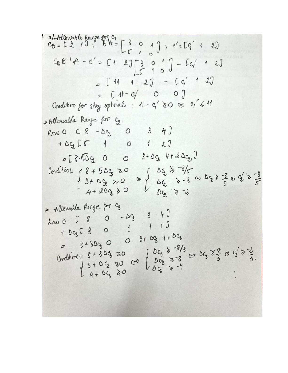
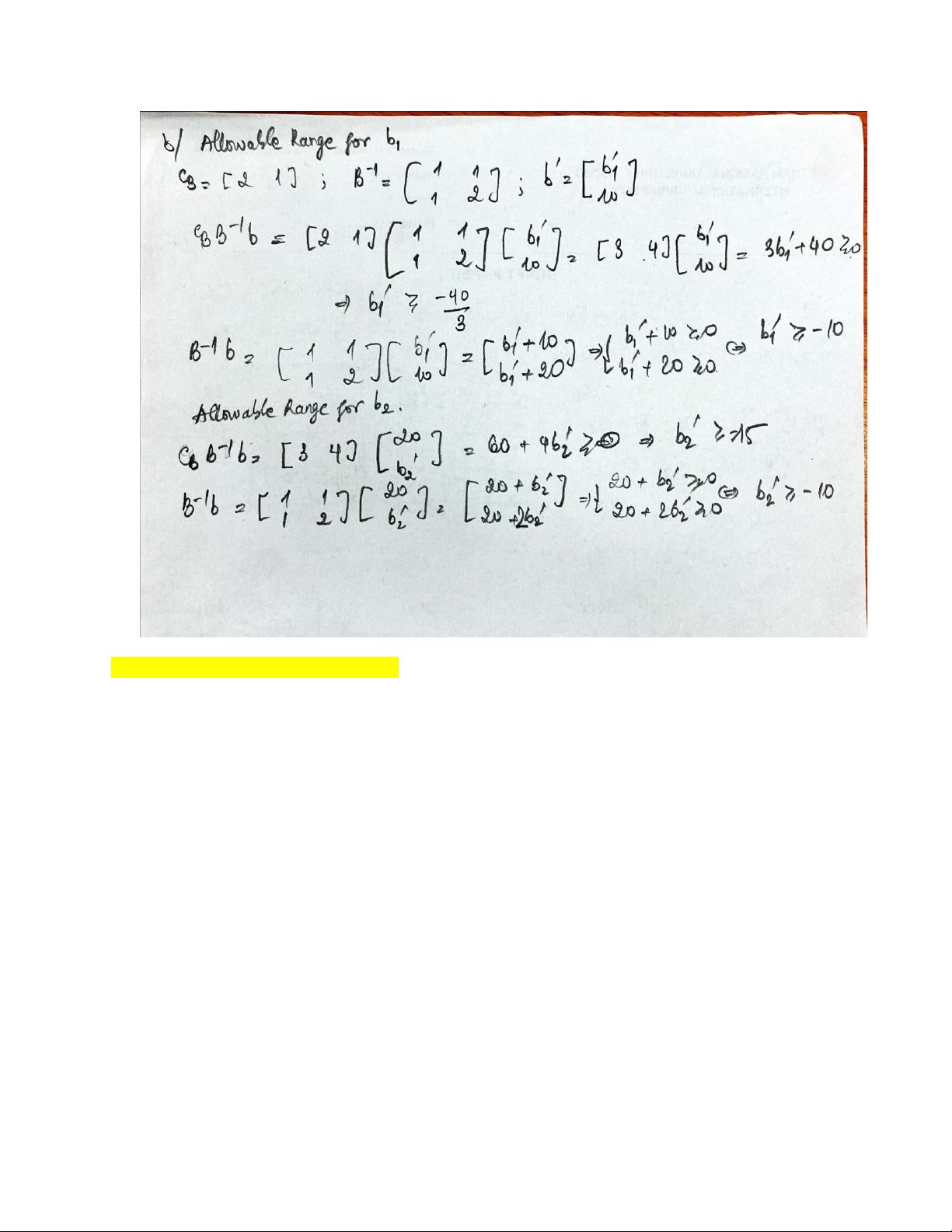
method, the final simplex tableau is: Basic Coefficient of: variable Eq. x_1 x_2 x_3 x_4 x_5 RHS Z (0) 8 0 0 3 4 100 x_3 (1) 3 0 1 1 1 30 x_2 (2) 5 1 0 1 2 40
a. Use algebraic analysis to find the allowable range to stay optimum for each c j
b. Use algebraic analysis to find the allowable range to stay feasible for each bi Solution:
a. Use algebraic analysis to find the allowable range to stay optimum for each c j lOMoAR cPSD| 58583460 lOMoAR cPSD| 58583460
Question 2 (change and check optimality)
Maximize Z=−5 x1+5 x2+13x3, subject ¿:
−x1+ x2+3 x3≤20 12
x1+4 x2+10 x3≤90 ¿ x j
≥0( j=1,2,3) .
If we let x4 and x5 be the slack variables for the respective constraints, the simplex method yields the
following final set of equations:
(0 ) Z+2 x3+5x4=100
(1)−x1+x2+3x3+x4=20
(2) 16 x1−2x3−4 x4+x5=10
Now you are to conduct sensitivity analysis by independently investigating each of the following changes
in the original model. For each change, use the sensitivity analysis procedure to revise this set of equations
(in tableau form) and convert it to proper form from Gaussian elimination for identifying and evaluating
the current basic solution. Then test this solution for feasibility and for optimality. (Do not reoptimize.) a.
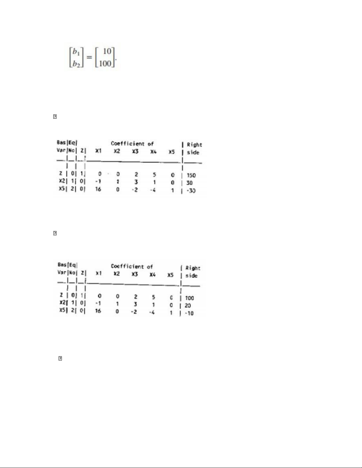
Change the right-hand side of constraint 1 to b1=30. b.
Change the right-hand side of constraint 2 to b2=70 c.
Change the right-hand sides to lOMoAR cPSD| 58583460 d.
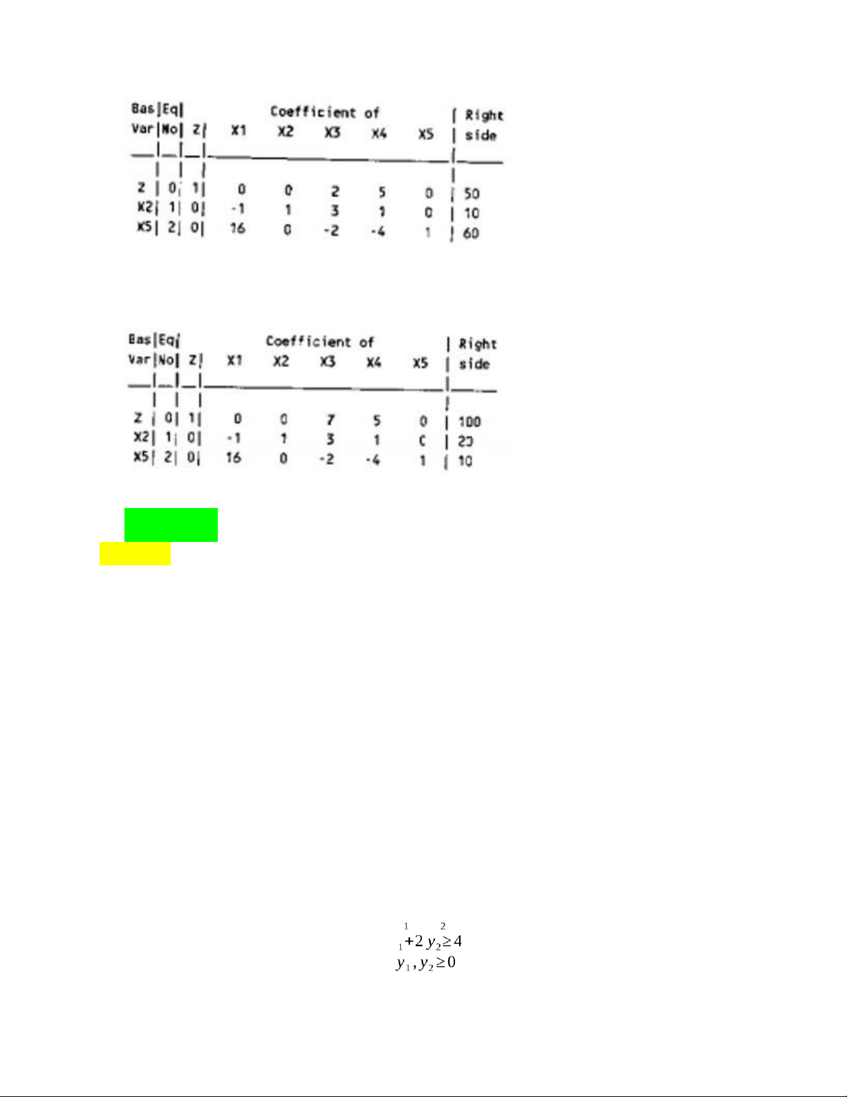
Change the coefficient of x3 in the objective function to c3=8 Solution: a. Δb1=10, Δb2=0 1)(10)=−40
ΔZ¿=(5 0 )(10)=50; Δb ¿1=(1 0)(100 )=10; Δb¿2=(−4 0 0 New table:
The current basic solution is infeasible b.
Δb1=0, Δb2=−20 ΔZ¿=(5 0 )( 020)=0; Δb ¿ ¿
1 =(1 0)( 020)=0; Δb2 =(−4 1)(10)=−20 − − 0 New table:
The current basic solution is infeasible.
c. Δb1=−10, Δb2=10 10 10
ΔZ¿=(5 0 )(−1010)=−50; Δ b¿ ) ¿ ) 1=(1 0)(−10
=−10; Δb2 =(−4 1)(−10 =50 New table: lOMoAR cPSD| 58583460
The current basic solution is feasible and optimal d. Δc3=−5 New table:
The current basic solution is feasible and optimal. II. Duality Question 3:
Consider the following problem
Maximize Z=2x1+7 x2+4 x3
subject ¿: x1+2x2+x3≤10
3 x1+3 x2+2x3≤10 ¿
x1, x2, x3≥0
a. Construct the dual problem for this primal problem
b. Use the dual problem to demonstrate that the optimal value of Z for the primal problem cannot exceed 25.
c. Solve the dual problem graphically. Use this solution to identify the basic variables and the
nonbasic variables for the optimal solution of the primal problem. Directly derive this solution, using Gaussian elimination. Solution: a.
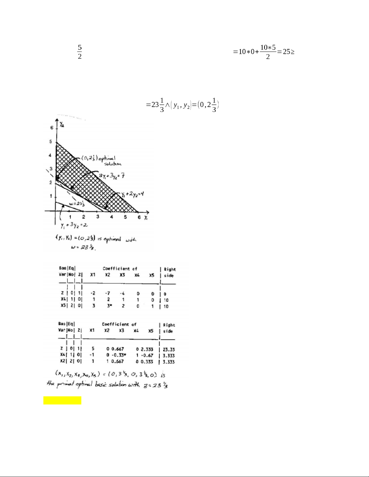
MinimizeW=10 y1+10 y2 subject ¿
y1+3 y2≥2
2 y +3 y ≥7 y lOMoAR cPSD| 58583460
b. (0, ) is feasible for the dual problem. Using weak duality, w Z. So, the
optimal primal objective value is less than 25
c. From the dual solution y2, y3∧y5 are basic, therefore, x3,x5∧x1 are non-basic primal variable, x2∧x4 are basic.
Graphical solution of dual problem: W Using Gauss elimination: Question 4: Consider the following problem: lOMoAR cPSD| 58583460
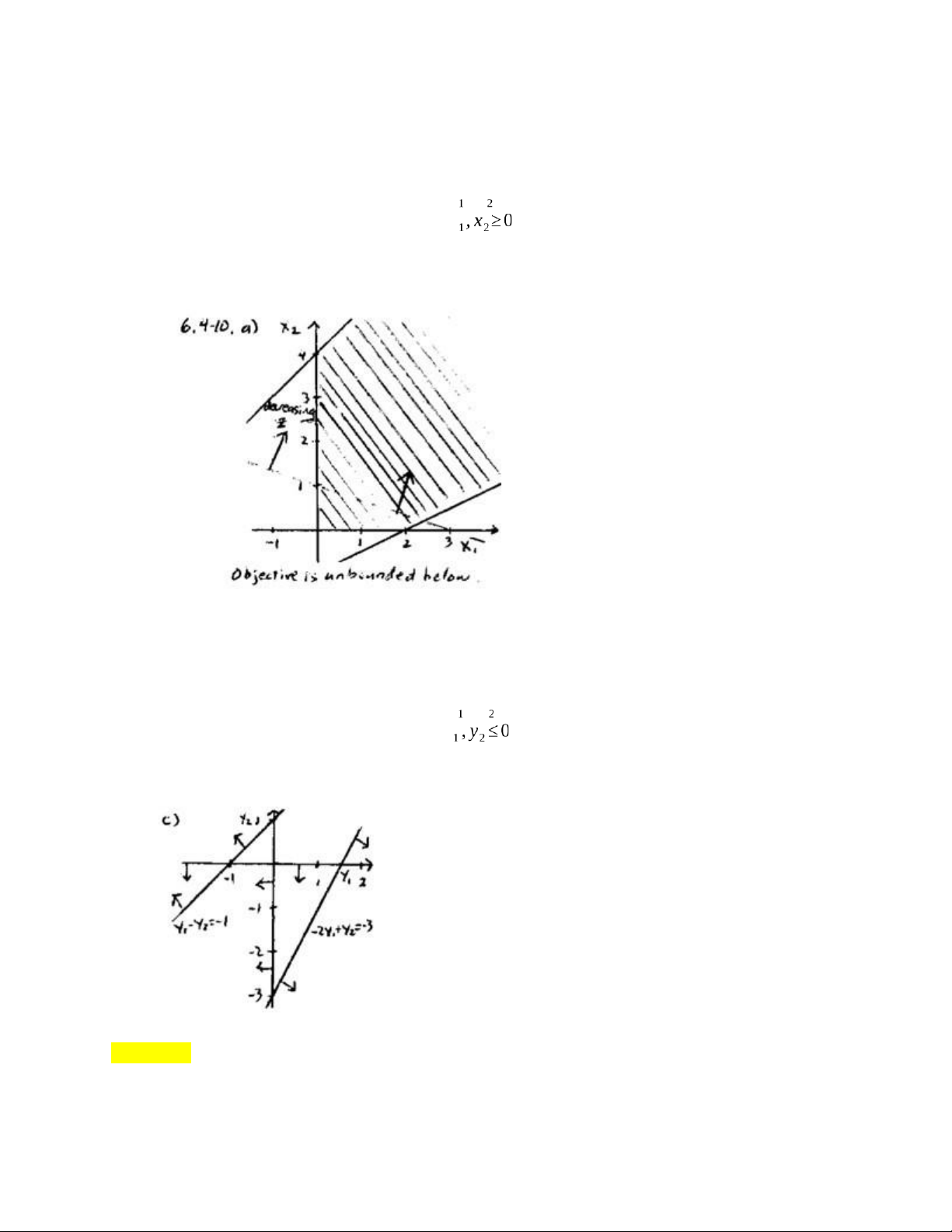
Minimize Z=−x1−3 x2 subject ¿:
x1−2 x2≤2 −x + x ≤4 ¿ x
a. Demonstrate graphically that this problem has an unbounded objective function b. Construct the dual problem
c. Demonstrate graphically that the dual problem has no feasible solutions. Solution: a. b. Dual:
Maximize2 y1+4 y2 subject ¿
y1−y2≤−1 −2 y + y ≤−3 y
c. As can be seen by the figure below, the dual problem has no feasible solution Question 5:
Consider the following problem: lOMoAR cPSD| 58583460
Maximize Z=3 x1+x2+4 x3, subject¿
6 x1+3x2+5 x3≤25
3 x1+4 x2+5x3≤20 x1,
x2, x3≥0
The corresponding final set of equations yielding the optimal solution is:
x1, x2, x3≥0
a. Identify the optimal solution from this set of equations. b. Construct the dual problem
c. Identify the optimal solution for the dual problem from the final set of equations. Verify this
solution by solving the dual problem graphically.
d. Suppose that the original problem is changed to
Maximize Z=3 x1+3 x2+4 x3 subject¿
6 x1+2x2+5 x3≤25
3 x1+3 x2+5 x3≤20 x1,
x2, x3≥0
Use duality theory (refer section 6.5 - page 252 Hiller’s Book 7th ed) to determine whether the previous
optimal solution is still optimal
e. Now suppose that the only change in the original problem is that a new variable xnew has been
introduced into the model as follows:
Maximize Z=3 x1+x2+4 x3+2 xnew, subject¿
6 x1+3x2+5 x3+3 xnew ≤25 lOMoAR cPSD| 58583460
3 x1+4 x2+5x3+2 xnew≤20 x1,
x2, x3,xnew ≥0
Use duality theory (refer section 6.5 - page 252 Hiller’s Book 7th ed) to determine whether the previous
optimal solution, along with xnew=0, is still optimal. Solution:
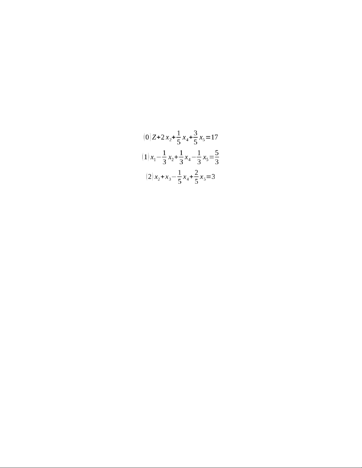
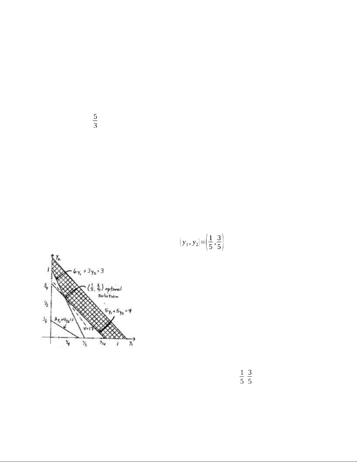
a. (x1,x2,x3)=( ,0,3) and Z=17 b. Dual problem:
MinimizeV =25 y1+20 y2 subject ¿:
6 y1+3 y2≥3
3 y1+4 y2≥1
5 y1+5 y2≥4 y1, y2≥0
c. The optimal solution for the dual problem is: and Z=17
d. Since the new dual constraint 2 y1+3 y2≥3 is violated for ( y1, y2)=( , ). The current
solution is no longer optimal.
e. The new primal variable adds a constraint to the dual: lOMoAR cPSD| 58583460
3 y1+2 y2≥2, which is not satisfied by (y1, y2¿=( , ). Therefore, the previous solution is no longer optimal.
Network optimization: shortest path problem, minimum spanning tree problem, maximum flow problem, minimum cost flow problem.
CHAPTER 7: Integer Programming Integer programming I. Question 1 (formulation):
The board of directors of General Wheels Co. is considering seven large capital investments. Each
investment can be made only once. These investments differ in the estimated long-run profit (net present
value) that they will generate as well as in the amount of capital required, as shown by the following table
(in units of millions of dollars): Investment Opportunity 1 2 3 4 5 6 7 Estimated profit 17 10 15 19 7 13 9 Capital required 43 28 34 48 17 32 23
The total amount of capital available for these investments is $100 million. Investment opportunities 1
and 2 are mutually exclusive, and so are 3 and 4. Furthermore, neither 3 nor 4 can be undertaken unless
one of the first two opportunities is undertaken. There are no such restrictions on investment
opportunities 5,6 and 7. The objective is to select the combination of capital investments that will
maximize the total estimated long-run profit (net present value).
Formulate a BIP model for this problem. Solution
Let xi: Binary variable (0,1), xi=1 if invest in opportunities i. Otherwise, xi=0 for i=1,…,7 pi:
Estimated profit of opportunities i for i=1,…,7 ci: Capital required by opportunities i for i=1,…,7 7
Maximize Z=∑ xi pi i=1 subject ¿ 7
∑ x c ≤100,∀i=1,…,7 i lOMoAR cPSD| 58583460
x1+x2≤1; x3+ x4≤1
x3≤ x1+x2 x4≤x1+x2
xi∈ (0,1) ,∀i=1,…,7 Question 2 (Formulation)
The Research and Development Division of the Progressive Company has been developing four possible
new product lines. Management must now make a decision as to which of these four products actually
will be produced and at what levels. Therefore, an operations research study has been requested to find
the most profitable product mix.
A substantial cost is associated with beginning the production of any product, as given in the first row of
the following table. Management’s objective is to find the product mix that maximizes the total profit
(total met revenue mis start-up costs) Product 1 2 3 4 Start-up cost $50,000 $40,000 $70,000 $60,000 Marginal revenue $70 $60 $90 $80
Let the continuous decision variables x1, x2, x3 and x4 be the production levels of products 1,2,3 and 4,
respectively. Management has imposed the following policy constraints on these variables:
1. No more than two of the products can be produced.
2. Either product 3 or 4 can be produced only if either product 1 or 2 is produced.
3. Either 5 x1+3 x2+6 x3+4 x4≤6,000
Or 4 x1+6 x2+3 x3+5 x4≤6,000
Introduce auxiliary binary variables to formulate a mixed BIP model for this problem Solution
Let yi : Binary variable (0,1) yi=1 if deciding to produce product i. Otherwise yi=0 (i=1,…4¿ u: Binary
variable (supporting constraint 3)
Ci: Cost to setup the production line for product i (Start-up cost) (i=1,…4¿ Ri: Unit
revenue of product i (Marginal revenue) (i=1,…4¿ 4
Maximize Z=∑ Ri xi−Ci yi i=1 subject¿ lOMoAR cPSD| 58583460
y1+y2+ y3+ y4≤2
y3≤ y1+y2 y4≤ y1+ y2
5 x1+3 x2+6 x3+4 x4≤6,000+uM
4 x1+6 x2+3 x3+5 x4≤6,000+M(1−u) x ≤ M y ,i=1,…4 x:Bignumber II.
Branch and Bound problem (BIP and MIP)
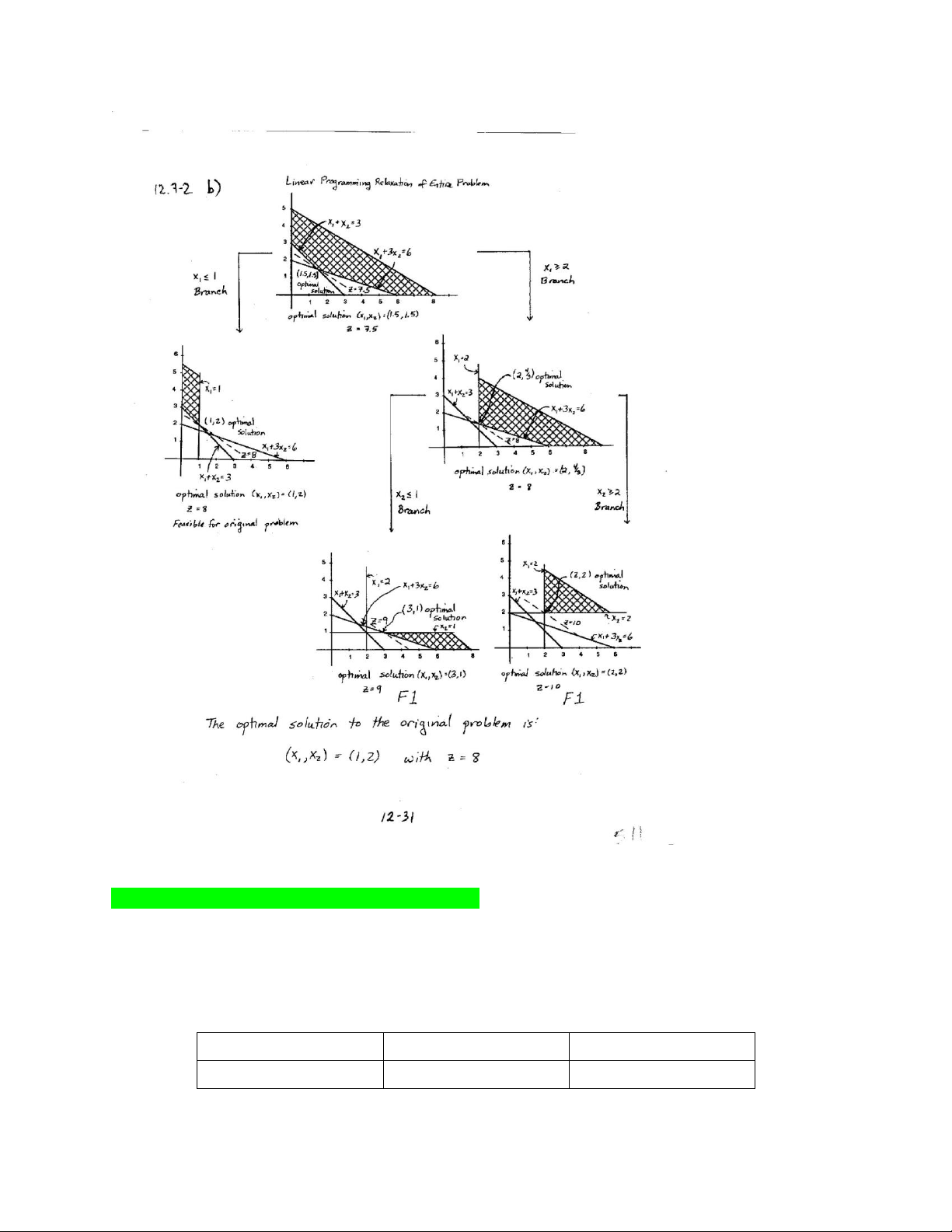
Question 3: (MIP) Solve the following Integer Programming (IP) problem using Branch and Bound algorithm:
Minimize Z=2 x1+3 x2, subject¿
x1+x2≥3 x1+3x2≥6
¿ x1≥0, x2≥0:x1,x2 are integers Solution: lOMoAR cPSD| 58583460
CHAPTER 8: Dynamic Programming
Dynamic programming problems: Knap-sack problem
Minh, a Vietnamese athlete who visits the United States and Europe frequently, is allowed to return with
a limited number of consumer items not generally available in Vietnam. The items, which are carried in a
duffel bag, cannot exceed a weight of 5 pounds. Once Minh is in Vietnam, he sells the items at highly
inflated prices. The three most popular items in Vietnam are denim jeans, CD players, and CDs of U.S. rock
groups. The weight and profit (in U.S. dollars) of each item are as follows: Item Weight (lb.) Profit Denim jeans 2 $90 lOMoAR cPSD| 58583460 CD players 3 150 Compact discs 1 30
Help Minh determine the combination of items he should pack in his duffel bag to maximize his profit. Solution: Weight 0 1 2 3 4 5 Item 0 0 0 0 0 0 0 1 0 0 90 90 90 90 2 0 0 90 150 150 240 3 0 30 30 150 180 240
Select item 1 and 2 or Denim jeans and CD players get the optimal profit
CHAPTER 9: Network Optimization III. Network optimization Shortest path problem: Question 1:
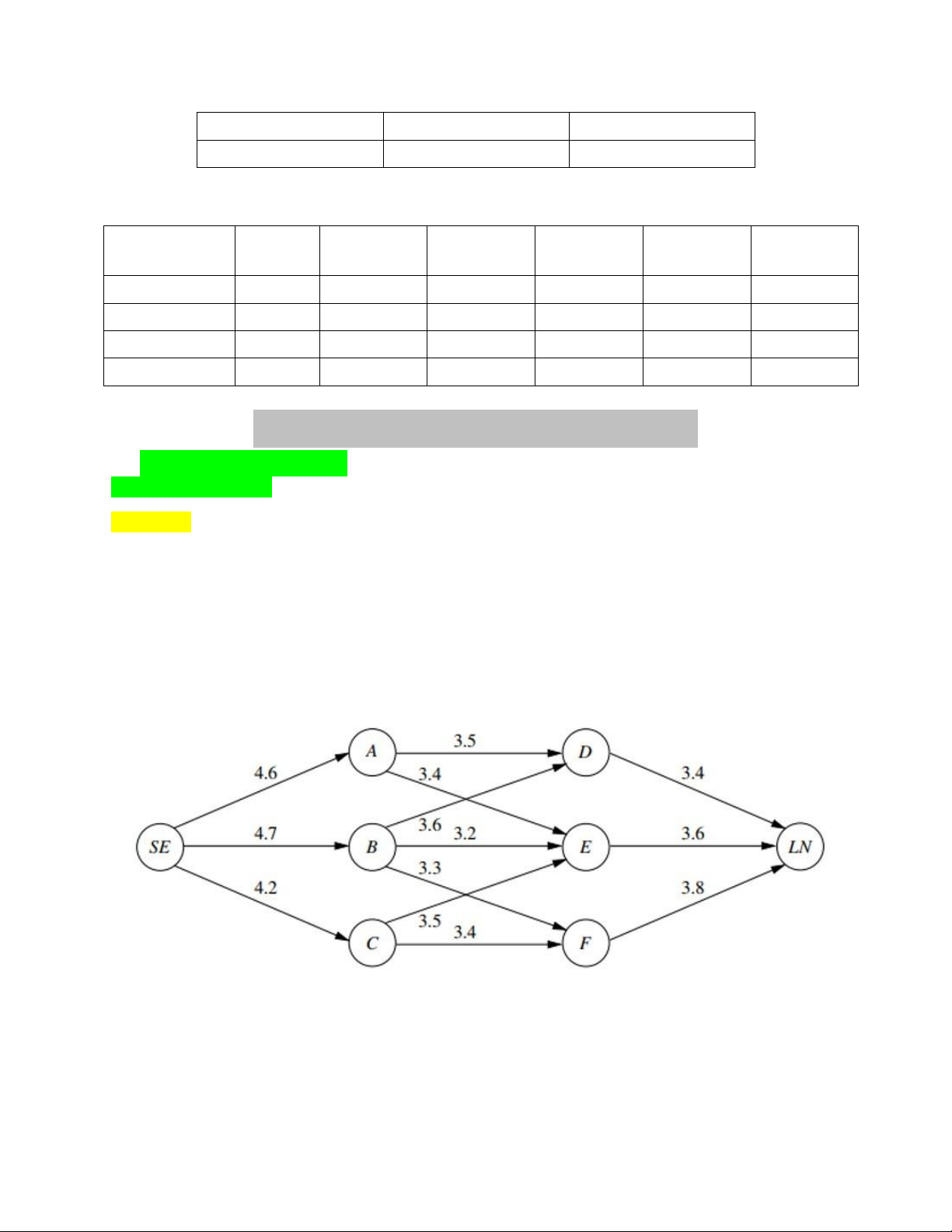
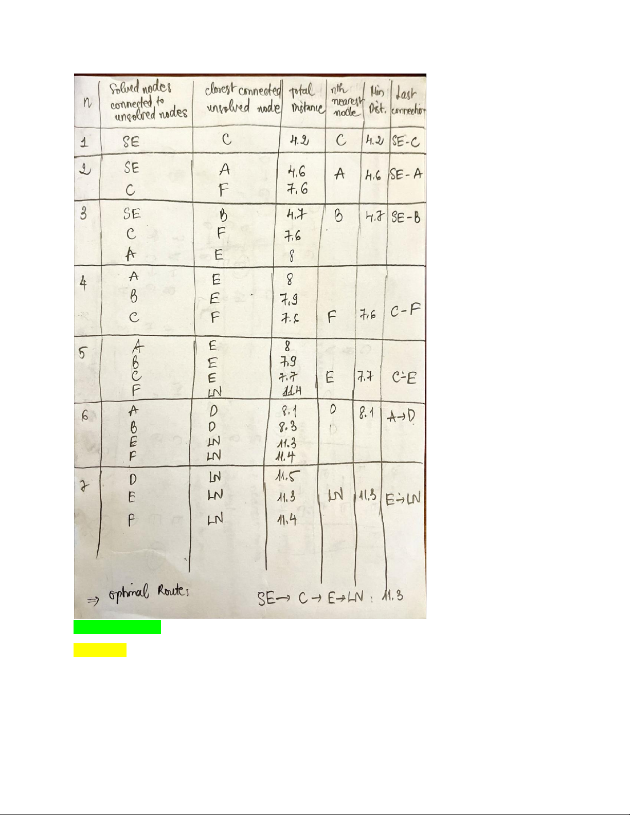
One of Speedy Airlines’ flights is about to take off from Seattle from a nonstop flight to London. There is
some flexibility in choosing the precise route to be taken, depending upon weather conditions. The
following network depicts the possible routes under consideration, where SE and LN are Seattle and
London, respectively, and the other nodes represent various intermediate locations. The winds along each
arc greatly affect the flying time (and so the fuel consumption). Based on current meteorological reports,
the flying times (in hours) for this particular flight are shown next to the arcs. Because the fuel consumed
is so expensive, the management of Speedy Airlines has established a policy of choosing the route that
minimizes the total flight time.
Use the algorithm described in Sec. 9.3 (Hiller’s Book 7th Edition) to solve this shortest path problem. Solution: lOMoAR cPSD| 58583460 Dijkstra’ algorithm: Question 2:
The network in the figure below gives the distances in miles between pairs of cities 1, 2, …, and 8. Use
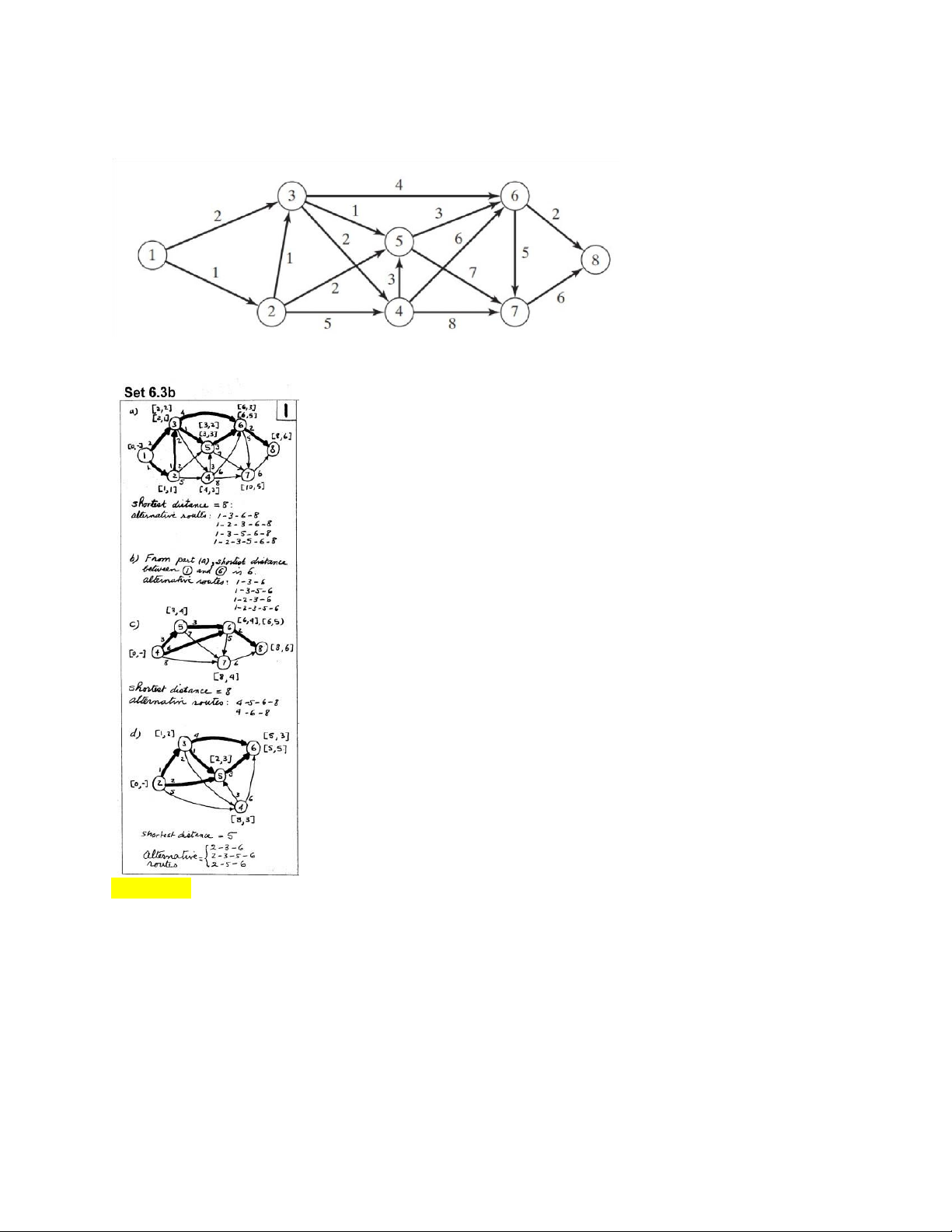
Dijkstra’s algorithm to find the shortest route between the following cities: a. Cities 1 and 7. b. Cities 1 and 6 lOMoAR cPSD| 58583460 c. Cities 4 and 8 d. Cities 2 and 7 Solution: Question 3:
Use Dijkstra’s algorithm to find the shortest route between node 1 and every other node in the network of the figure below: lOMoAR cPSD| 58583460 Solution: Minimum spanning tree: Question 4:
Midwest TV Cable Company is providing cable service to five new housing developments. The figure below
depicts possible TV connections to the five areas, with cable miles affixed on each arc.
The goal is to determine the most economical cable network. Determine the minimal spanning tree of the
network under each of the following separate conditions:
a. Nodes 5 and 6 are linked by a 2-mile cable
b. Nodes 2 and 5 cannot be linked lOMoAR cPSD| 58583460
c. Nodes 2 and 6 are linked by a 4-mile cable
d. The cable between nodes 1 and 2 is 8 miles long.
e. Nodes 3 and 5 are linked by a 2-mile cable.
f. Node 2 cannot be linked directly to nodes 3 and 5. Solution:
Spanning tree length = 16 where N2-N5 (5 miles) , N1-N2 (1), N4-N2 (4), N6-N4 (3), N3-N4 (5)
a. Spanning tree length = 14 where N2-N1 (1), N5-N2(3), N6-N5(2), N4-N6(3), N3-N4(5)
b. Spanning tree length = 21 where N2-N1(1), N4-N2(4), N6-N4(3), N3-N4(5), N5-N4 (8)
c. Spanning tree length = 16 where N2-N1(1), N5-N2(3), N6-N2 (4), N4-N6 (3), N3-N4(5)
d. Spanning tree length = 20 where N3-N1(5), N4-N3(5), N6-N4 (3), N2-N4 (4), N5-N2(3)
e. Spanning tree length = 13 where N2-N1(1), N5-N2 (3), N3-N5 (2), N4-N2 (4), N6-N4 (3)
f. Spanning tree length = 21 where N2-N1(1), N4-N2(4), N6-N4 (3), N3-N4 (5), N3-N4(5), N5-N4 (8)
Minimum cost flow _ Maximum flow: Question 5:
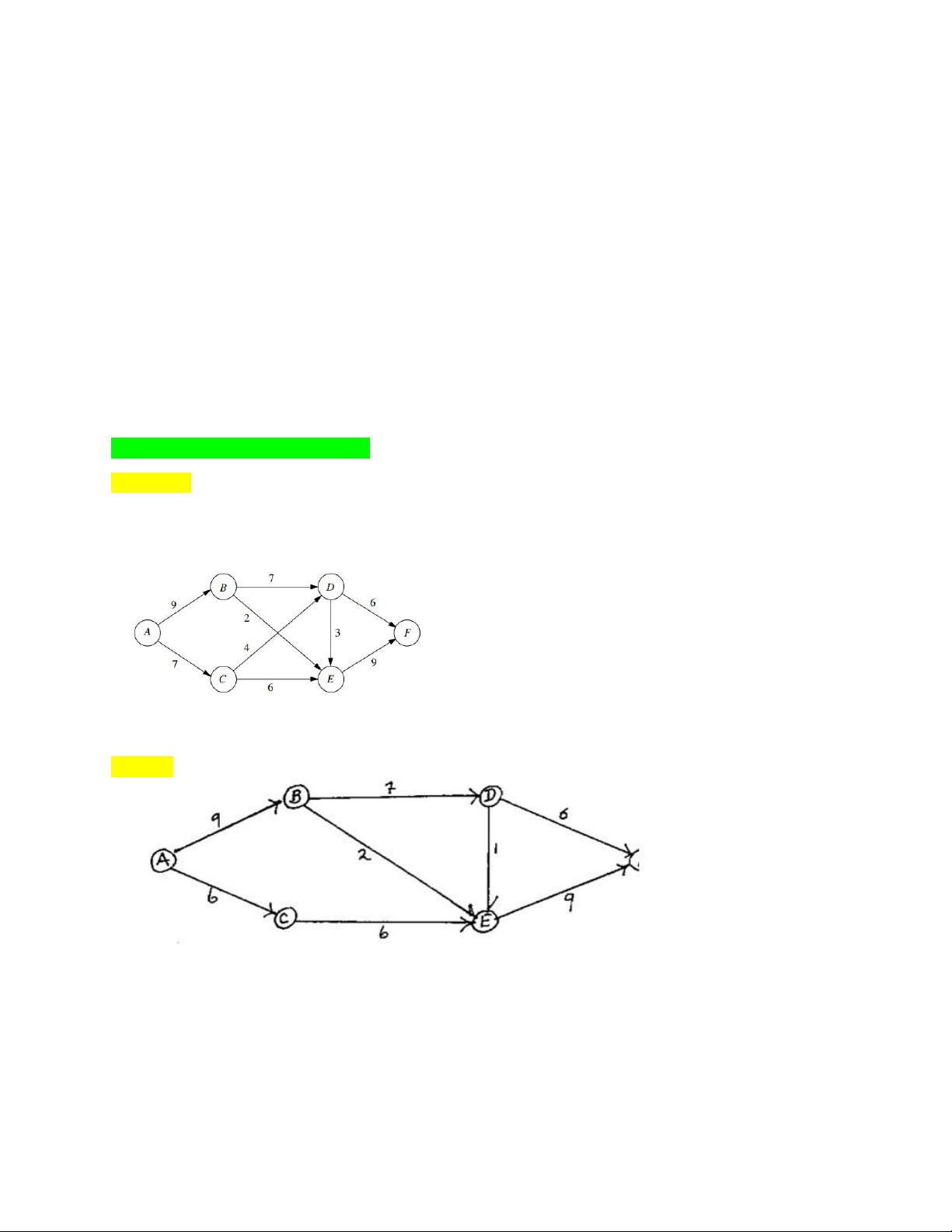
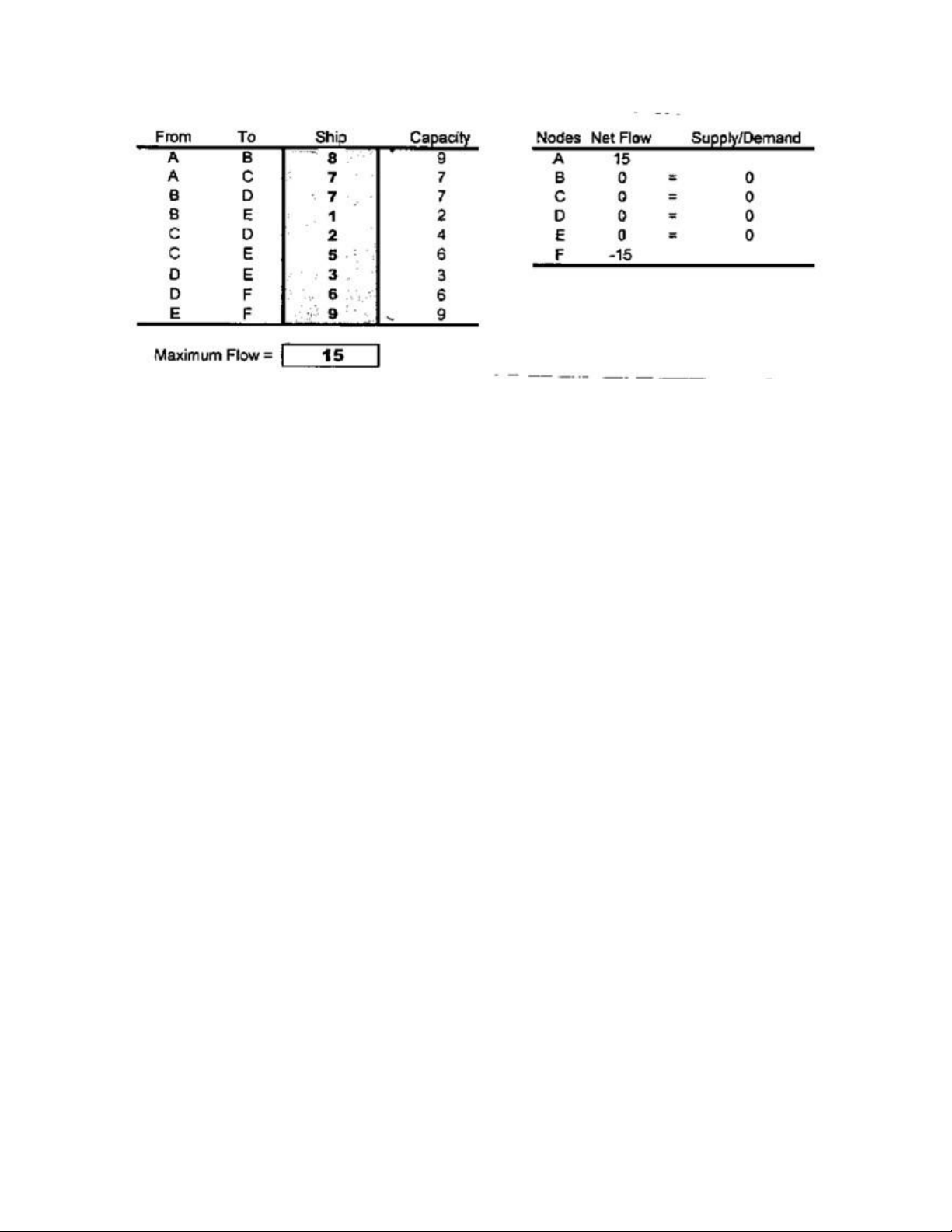
Consider the maximum flow problem shown below, where the source is node A, the sink is node F, and
the arc capacities are the numbers shown next to these directed arcs.
Use the augmenting path algorithm (Maximum flow problem) to solve the problem. Solution: lOMoAR cPSD| 58583460 lOMoAR cPSD| 58583460
Chapter 10: Non-linear programming Non-linear programming
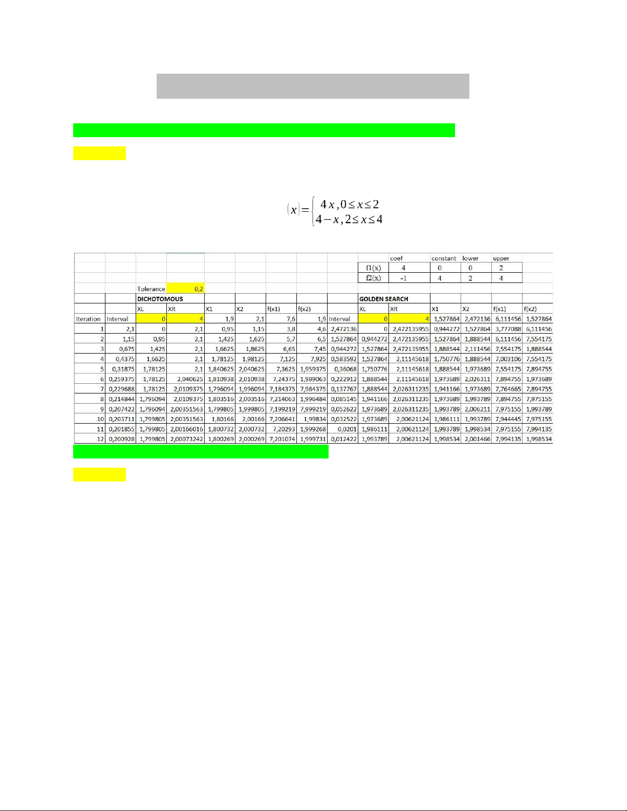
Non-linear programming (Single variable)- Dichotomous and Golden search method Question 1:
Find the maximum of each of the following functions by dichotomous search. Assume that Δ=.2: f Solution:
Unconstrained – Multivariable: Gradient Search method Question 2:
Starting from the initial trial solution (x1,x2)=(0,0), interactively apply the gradient search procedure with
ϵ=0.3 to obtain an approximate solution for the following problem, and then apply the automatic routine
for this procedure (with ϵ=0.01)
Maximize f ( x )=8x1−x21−12 x2−2 x22+2 x1x2
Then solve ∇ f ( x )=0 directly to obtain the exact solution Solution: