Final Exam - Business Computing Skills | Trường Đại học Quốc tế, Đại học Quốc gia Thành phố HCM

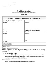
International University - VNUHCM
School of Business Administration ----------------- Final Examination
Date: 15/01/2022; Duration: 120 minutes
Open book; Online; Laptops are allowed.
SUBJECT: Business Computing Skills (ID: BA120IU)
Approval by the School of Business Administration Lecturer: Signature Signature Full name:
Full name: Dr. Nguyen Ngoc Truong Minh Proctor 1 Proctor 2 Signature Signature
Full name: Nguyen Ngoc Truong Minh Full name: STUDENT INFO
Student name: __________________
Student ID: __________________
INSTRUCTIONS: the total of point is 100 (equivalent to 40% of the course) 1. Purpose:
• Test your knowledge in CLO6
• Examine your skill in analysis and preparing documents, presentations, and spreadsheets
• Examine your skill in filing and scheduling management skills to support management and supervisors 2. Requirements:
• Carefully read each question and answer it following the requirements
• There are two parts: Part 1 20% (20 Multiple-Choice Questions) doing directly on Blackboard
using the link given by the instructor; Part 2 80% (08 MS Excel exercises) doing on your computer
and submit your exam on Blackboard (Assignment rubric)
• This exam paper contains 07 pages in total
International University – VNUHCM
Student Name:………...………….
School of Business Administration Student ID:………………………. -----------------
PART 1: MULTIPLE CHOICE QUESTIONS (20%) PART 2: EXCEL (80%)
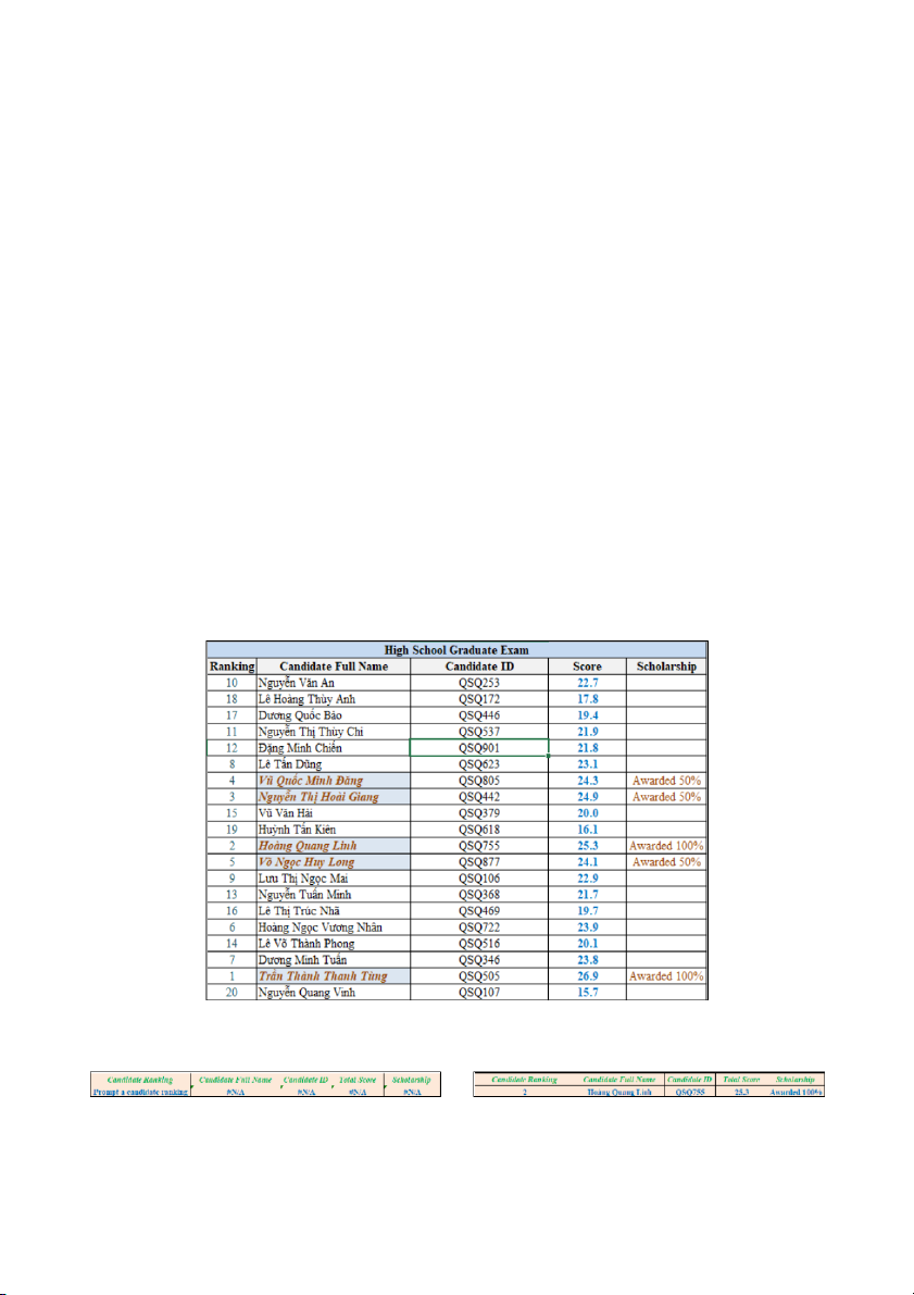
I. Formulas and Conditional Formatting (20pts)
- In the BonusScore workbook, fill the bonus score in the Score column (column B) for each candidate
based on their zone of residence with the following rules (noted that the zones are given as text): (2pts) • Zone “A”: no bonus point •
Zone “B”: bonus 0.1 points •
Zone “C”: bonus 0.2 points
- Open the file Problem1.xlsx
- From this time forth, work only in Problem1.xlsx: first of all, use the data in four workbooks
(MathsScore, EnglishScore, ScienceScore and BonusScore) to calculate the Total Score (column D)
applying the given formula, display the result with 1 decimal place: (5pts)
Total Score = Maths + English + Science + Bonus
- Use Conditional Formatting to highlight all the candidates’ full name (Light Blue Fil with Dark Orange,
Bold Italic Text) whose total score (column D) is greater than or equal to 24.0 (4pts)
- Use RANK function to rank all the candidates (column A) in the list based on their Total Score (2pts)
- Use IF and CONCATENATE functions to fill the Scholarship column (column E) the text “Awarded
…%” for Top-5 candidates (rank 1-2: 100%, rank 3-5: 50%), others leave the field empty (3pts).
- Use VLOOKUP functions to fill the information in the orange table while inputting a candidate ranking
as example below (4pts). ð 2/7
International University – VNUHCM
Student Name:………...………….
School of Business Administration Student ID:………………………. ----------------- ACBSP: Reflective thinking
Topic: MS Excel - Using Basic Formulas & Advanced Formulas
Bloom’s Taxonomy: Application, Synthesis
Relevant Program Learning Outcomes: PO3, PO5
Relevant Course Learning Outcomes: CLO6
Level of Difficulty: 2 Average II. Basic Chart (8pts)
- Open the file Problem2.xlsx
- Plot two charts like Fig.2 in the active worksheet.
- Chart type: 3-D Pie, chart style: Style 5
- Text font: Arial, bold, font size: chart title 16, data labels 10.
- Angle of first slice (North region): 90°.
- Two slices South and International are pulled out from the others. Expenses Revenue West, $12,842,000 , West, 15% East, $26,795,000 , East, International, $43,323,000 , 19% $34,296,000 , $8,473,000 , 31% International, 40% 10% $7,494,000 , 5% North, $9,927,000 , North, 12% $27,356,000 , 20% South, South, $19,392,000 , $34,523,000 , 23% 25%
Fig.2 - Brigham Corporation Expenses and Revenue by Regions. ACBSP: Reflective thinking Topic: MS Excel - Charting
Bloom’s Taxonomy: Understanding, Application
Relevant Program Learning Outcomes: PO3, PO5
Relevant Course Learning Outcomes: CLO6
Level of Difficulty: 1 Easy
III. Trend-Line (12pts )
- Open the file Problem3.xlsx
- Plot a scatter diagram in a new worksheet which names Problem3_Chart.
- For the whole chart, use chart style: Style 6, text font: Book Antiqua, bold, font size: chart title 20,
legends and axis titles 16, other elements 12, add also Minor Gridlines to both Horizontal and Vertical
as shown in Fig.3 (note that all the gridline colors should be white, the width is 0.5pt).
- Modify each data and the marker to fit with its color (for red data, use a diamond õ as the marker, for
green data, use an asterisk þ as the marker, all are size: 9, remember that with red marker you need
to modify both marker fill and marker border line color).
- Add the trend-line to each data 5 periods forwards (for red data, trend-line type: Power, linewidth: 3/7
International University – VNUHCM
Student Name:………...………….
School of Business Administration Student ID:………………………. -----------------
2.5pt, dash type: dash, for green data, trend-line type: Logarithmic, linewidth: 2.5pt, dash type: dash
dot, color should be adapted to its data). Balloon Sold Red vs. Green Red Green Power (Red) Log. (Green) 150 120 A m ou 90 nt Chang 60 e 30 0 0 5 10 15 20 25 30 Months
Fig.3 - Balloon Sold Red vs. Green ACBSP: Reflective thinking
Topic: MS Excel – Charting and Trendlines
Bloom’s Taxonomy: Application, Synthesis
Relevant Program Learning Outcomes: PO3, PO5
Relevant Course Learning Outcomes: CLO6
Level of Difficulty: 3 Difficult
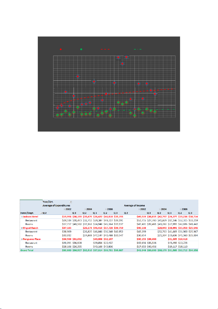
IV. PivotTable and PivotChart (20pts)
- Open the file Problem4.xlsx
- Check the data consistency – the three conditions – in order to create the PivotTable (2pts)
- Create a PivotTable in a new worksheet which names DataInPivotTable as in Fig4.1: (8pts)
Fig.4.1 - DataInPivotTable 4/7
International University – VNUHCM
Student Name:………...………….
School of Business Administration Student ID:………………………. -----------------
- Create a PivotChart in a new worksheet named Problem4_PivotChart (then move chart to another
new worksheet which names DataInPivotChart) as shown in Fig4.2, chart type: 3-D Clustersed
Column, chart style: Style 5, text font: Verdana, bold, font size: chart title 16, other elements 12, add
Minor Gridlines to Horizontal axis, 3-D rotation X-axis 30ç, Y-axis 30ç (10pts)
Total Expenditures in Three hotel branches in the First
Quarter Q1 through five years 2002-2006 2002 40 2003 2004 35 2005 x 10000 30 2006 25 20 15 10 5 0 Q 1 Q 1 Q 1 Jackson Hotel Miguel Ranch Pengueno Place
Fig.4.2 - DataInPivotChart ACBSP: Reflective thinking
Topic: MS Excel – Pivoting Data
Bloom’s Taxonomy: Application, Synthesis
Relevant Program Learning Outcomes: PO3, PO5
Relevant Course Learning Outcomes: CLO6
Level of Difficulty: 2 Average
V. Sorting and Filtering Data (5pts)
- Open the file Problem5.xlsx
- Apply quick filters to find out all students considered as Asian, Black, Hispanic, Indian and White
(Ethnicity column has a value A, B, H, I and W ³ 3162 records found) who have M-E (column P) less
than 30 (1433 records found), then R-M (column U) is in the range from 30 to 80 (1120 records found).
- After that, sort the students in Ethnicity as the following order: A, I, W, H then B. Next, add a second
level of sorting in descending order of M-A. At the end, add a third level of sorting in ascending order of W-A. ACBSP: Reflective thinking
Topic: MS Excel - Using Basic Formulas & Advanced Formulas
Bloom’s Taxonomy: Application, Synthesis
Relevant Program Learning Outcomes: PO3, PO5
Relevant Course Learning Outcomes: CLO6 Level of Difficulty: 1 Easy 5/7
International University – VNUHCM
Student Name:………...………….
School of Business Administration Student ID:………………………. -----------------
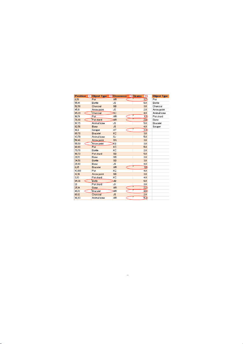
VI. Validating Data (5pts)
- Open the file Problem6.xlsx
- Use Data Tools to remove the duplicate data in Object Type (column F)
- Use Data Validation to circle all cells in column B (Object Type - from row 2 to row 31) that do not
belong to the valid list (List of Object Type)
- Create an input message (Title: Object Type, Input Message: “Values only in the Object Type list.”)
and an error alert (Style: Warning, Title: Not allowed value, Error message: “Invalid!!! Values only in
the Object Type list.”)
- Use Data Validation to restrict text length of all cells in column C (Discoverer) to 2 characters only
and circle all cells that are not positive integer numbers (whole numbers) in column D (Grams) ACBSP: Reflective thinking
Topic: MS Excel – Data Validation
Bloom’s Taxonomy: Application, Synthesis
Relevant Program Learning Outcomes: PO3, PO5
Relevant Course Learning Outcomes: CLO6
Level of Difficulty: 2 Average
VII. What-If Analysis – Scenario Manager (7pts)
- Open the file Problem7.xlsx (sheet Expected Income)
- The manager of the restaurant wants to apply a new business strategy plan in order to increase the
annual profit of the restaurant as follows (Scenario Manager named New business plan): 
• In the first four months (Jan-Apr): To-Go Orders = *Eat-In Orders 
• In the next two months (May-Jun): Eat-In Orders = 12*To-Go Orders 6/7
International University – VNUHCM
Student Name:………...………….
School of Business Administration Student ID:………………………. ----------------- 
• In the next three months (Jul-Sep): To-Go Orders = *Eat-In Orders  24
• In the last three months (Oct-Dec): Eat-In Orders = *To-Go Orders
- Create a scenario to see how this business operation would affect the annual profit (create a summary
- DO NOT SHOW!!!). (Result: $179,004) ACBSP: Reflective thinking
Topic: MS Excel – What-If Analysis Scenario Manager
Bloom’s Taxonomy: Application, Synthesis
Relevant Program Learning Outcomes: PO3, PO5
Relevant Course Learning Outcomes: CLO6
Level of Difficulty: 2 Average
VIII. What-If Analysis – Goal Seeking (3pts)
- Open the file Problem8.xlsx
- Currently, the restaurant gets the annual profit $64,400 (sheet Expected Income). However, the
managers want more than that, they want to increase the profit up to $83,000 per year.
- Use Goal Seek to find out what is the new Benefit amount (sheet Average Expenses per month) that
the managers would apply in order to achieve the financial target set. Display with one decimal place
format and explain briefly about the result in the active worksheet. ACBSP: Reflective thinking
Topic: MS Excel – What-If Analysis Goal Seek
Bloom’s Taxonomy: Understanding
Relevant Program Learning Outcomes: PO3, PO5
Relevant Course Learning Outcomes: CLO6 Level of Difficulty: 1 Easy – END – 7/7