1 TR¯¡NG THANH HOA – MATHEMATICS FOR BUSINESS
CHAPTER 5: PARTIAL DIFFERENTIATION
1. FUNCTIONS OF SEVERAL VARIABLES
- Demand may depend on the price of the good and the income level of the consumer. Qd = f(P, Y)
- Output of a firm depends on inputs into the production process like capital and labour. Q = f(K, L)
1.1. First-order derivatives of a functions of 2 variables
- Differentiate with respect to x holding z constant: �㔕þ �㔕ý = Ąý
- Differentiate with respect to z holding x constant: �㔕þ �㔕ÿ = Ąÿ
Example: Find expressions for the first-order partial derivatives for the functions a) f(x, y) = 5x4 – y2
Differentiating 5x4 with respect to x gives 20x3 and, since y is held constant, y2 differentiates to zero. Hence �㔕Ą
�㔕ý = 20ý3 2 0 = 20ý3
Differentiating 5x4 with respect to y gives zero because x is held fixed. Also differentiating y2
with respect to y gives 2y, so �㔕Ą
�㔕þ = 0 2 2þ = 22þ b) f(x, y) = x2y3 – 10x
To differentiate the first term, x2y3, with respect to x we regard it as a constant multiple of x2
(where the constant is y3), so we get 2xy3. The second term obviously gives -10, so �㔕Ą �㔕ý = 2ýþ3 2 10
To differentiate the first term, x2y3, with respect to x we regard it as a constant multiple of x2
(where the constant is y3), so we get 2xy3. The second term obviously gives -10, so
2 TR¯¡NG THANH HOA – MATHEMATICS FOR BUSINESS �㔕Ą
�㔕þ = 3ý2þ2 2 0 = 3ý2þ2
1.2. Second-order derivatives of a functions of 2 variables - With y = f(x,z): �㔕2þ �㔕ý2 = Ąýý �㔕2þ �㔕ÿ2 = Ąýý �㔕2þ �㔕ý�㔕ÿ = Ąýÿ �㔕2þ �㔕ÿ�㔕ý = Ąÿý
Example: Find expressions for the second-order partial derivatives of the functions: a) f(x,y) = 5x4 – y2 f 2 xx = 60x fyy = 2 fyx = fxy = 0 b) f(x,y) = x2y3 – 10x f 3 xx = 2y f 2 yy = 6x y f 2 yx = fxy = 6xy
Example: Find expressions for the partial derivatives f1, f11 and f21 in the case when f(x 5 2
1, x2, x3) = x1x2 + x1 – x2 x3 �㔕Ą Ą 4 1 = �㔕ý = ý2 + 5ý1 1 �㔕2Ą Ą 3 11 = �㔕ý 12 = 20ý1 �㔕2Ą Ą21 = �㔕ý = 1 2�㔕ý1
1.3. Interpretation of partial derivatives
- If x and z change simultaneously, the small increments formula:
3 TR¯¡NG THANH HOA – MATHEMATICS FOR BUSINESS �㔕þ �㔕þ
∆þ j�㔕ý∆ý +�㔕ÿ ∆ÿ
Example: If z = xy – 5x + 2y, evaluate: �㔕ÿ �㔕ÿ �㔕ý ÿÿĂ �㔕þ at the point (2, 6).
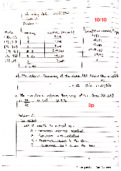
a) Use the small increments formula to estimate the change in z as x decreases from 2 to 1.9
and y increases from 6 to 6.1.
b) Confirm your estimate of part (a) by evaluating z at (2, 6) and (1.9, 6.1). �㔕ÿ �㔕ý = þ 2 5 �㔕ÿ �㔕þ = ý + 2 At (2, 6): �㔕ÿ �㔕ý = 1 �㔕ÿ �㔕þ = 4
a) ∆ý = 20.1, ∆þ = 0.1
ÿ ≅ 1(20.1) + 4(0.1) = 0.3, ĀĀ ÿ ÿÿāÿăÿĀăĀ Āþ ÿāāÿĀýÿþÿāăýþ 0.3.
b) At (2, 6), z = 14, and at (1.9, 6.1), z = 14.29, so the exact increase is 0.29.
1.4. Implicit Differentiation Ăþ Ąý Ăý = 2 Ą þ
Example: Use implicit differentiation to find expressions for dy/dx given that a) xy – y3 + y = 0 b) y5 – xy2 = 10 a) Ăþ 2þ Ăý = ý 2 3þ2 + 1 b)
4 TR¯¡NG THANH HOA – MATHEMATICS FOR BUSINESS Ăþ þ2 Ăý = 5þ4 2 2ýþ
2. APPLICATION I: ELASTICITY QUANTITY DEMANDED AS A FUNCTION OF SEVERAL VARIABLES
Ā� 㕑 = Ą(ÿ, ÿ�㔴, �㕌)
- Own price elasticity of demand:
ÿÿĀāĀÿāÿĀÿÿý ÿ/ÿÿąă ÿÿ ĀăþÿÿĂ
āÿ = ÿÿĀāĀÿāÿĀÿÿý ÿ/ÿÿąă ÿÿ ÿÿÿāă �㔕Ā ÿ āÿ = �㔕ÿ ýĀ
(Negative for a downward sloping demand curve).
- Cross price elasticity of demand:
ÿÿĀāĀÿāÿĀÿÿý ÿ/ÿÿąă ÿÿ ĀăþÿÿĂ
āÿ�㔴 =ÿÿĀāĀÿāÿĀÿÿý ÿ/ÿÿąă ÿÿ ÿÿÿāă ĀĄ ăĀĀĂ �㔴 �㔕Ā ÿ ā �㔴 ÿ�㔴 = ý �㔕ÿ� 㔴 Ā
(Negative for complements, positive for substitues).
- Income elasticity of demand:
ÿÿĀāĀÿāÿĀÿÿý ÿ/ÿÿąă ÿÿ ĀăþÿÿĂ ā� 㕌 =
ÿÿĀāĀÿāÿĀÿÿý ÿ/ÿÿąă ÿÿ �㔼ÿāĀþă �㔕Ā �㕌 ā� 㕌 = �㔕� Ā 㕌 ý
(Positive for normal goods, negative for inferior goods).
Example: Given the demand function:
Q = 500 – 3P – 2PA + 0.01Y
Where P = 20, PA = 30 and Y = 5000, find
(a) The price elasticity of demand.
(b) The cross-price elasticity of demand.
(c) The income elasticity of demand.
If income rises by 5%, calculate the corresponding percentage change in demand. Would this
good be classified as inferior, normal or superior?
5 TR¯¡NG THANH HOA – MATHEMATICS FOR BUSINESS
Substituing the given values of P, PA and Y into the demand equation gives
Q = 500 – 3 x 20 – 2 x 30 + 0.01 x 5000 = 430 a) �㔕Ā 20 ĀĀ �㔕ÿ = 23 āÿ = 430 ý (23) = 20.14 b) �㔕Ā 30 = 22 Ā ā Ā = �㔕ÿ ÿ� 㔴 � 㔴 430 ý (22) = 20.14 c) �㔕Ā 5000 ĀĀ = 0. �㔕�㕌 = 0.01 ā� 㕌 = 430 ý 0.01 12 By definition,
ÿÿĀāĀÿāÿĀÿÿý ÿ/ÿÿąă ÿÿ ĀăþÿÿĂ ā� 㕌 =
ÿÿĀāĀÿāÿĀÿÿý ÿ/ÿÿąă ÿÿ �㔼ÿāĀþă
So the demand rises by 0.12 x 5 = 0.6%. The good is normal since 0 < 0.6 < 1.
3. APPLICATION II: UTILITY
- Suppose there are two goods x1 and x2. The utility function relates the quantities of these
goods to the consumers levels of satisfaction using a utility function: Ą = Ą(ý1, ý2)
- Marginal utility associated with x1 (x2) gives the change in utility as a result of a one unit
change in the quantity of x1 (x2) consumed: �㔕Ą āĄ1 = �㔕ý 1 �㔕Ą āĄ2 = �㔕ý 2
- When both x1 and x2 change simultaneously, we can use the small increments formula to
determine the overall change in utility: �㔕Ą �㔕Ą ∆Ą j ∆ý �㔕ý 1 + ∆ý2 1 �㔕ý2
- We would expect the second derivative to be negative given the law of diminishing marginal utility:
6 TR¯¡NG THANH HOA – MATHEMATICS FOR BUSINESS �㔕2Ą �㔕2Ą �㔕ý12 < 0 ÿÿĂ �㔕ý22 < 0
Example: An individual’s utility function is given by U = 1000x 2 2
1 + 450x2 + 5x1x2 – 2x1 – x2
Where x1 is the amount of leisure measured in hours per week and x2 is earned income
measured in dollars per week. Determine the value of the marginal utilities. �㔕Ą �㔕Ą ÿÿĂ �㔕ý 1 �㔕ý2 When x1 = 138 and x2 = 500.
Hence estimate the change in U if the individual works for an extra hour, which increases
earned income by $15 per week.
Does the law of diminishing marginal utility hold for this function? �㔕Ą
�㔕ý = 1000 + 5ý2 2 4ý1 1 �㔕Ą
�㔕ý = 450 + 5ý1 2 2ý2 2 So at (138, 500): �㔕Ą �㔕Ą = 2948 ÿÿĂ = 140 �㔕ý 1 �㔕ý2
If working time increases by 1 hour then leisure time decreases by 1 hour, so ∆ý1 = 21. Also
∆ý2 = 15. By the small increments formula:
∆Ą = 2948 ý (21) + 140 ý 15 = 2848
The law of diminishing marginal utility holds for both x1 and x2 because �㔕2Ą �㔕2Ą �㔕ý12 = 24 < 0 ÿÿĂ �㔕ý22 = 22 < 0
- Indifference curves: displays all possible combinations of x1 and x2 that produce a constant level of utility. �㔕Ā Ăý2 �㔕ý1 Ăý = 2 1 �㔕Ā �㔕ý2
- Marginal rate of commodity substitution:
7 TR¯¡NG THANH HOA – MATHEMATICS FOR BUSINESS �㔕Ā Ăý �㔕 2 2 ý1 Ăý = 1 �㔕Ā �㔕ý2
Example: Calculate the value of MRCS for the utility function given in the above example at
the point (138, 500). Hence estimate the increase in earned income required to maintain the
current level of utility if leisure time falls by 2 hours per week. 2948 āāÿĂ = 140 = 21.06
This represents the increase in x2 required to maintain the current level of utility when x1 falls
by 1 unit. Hence if x1 falls by 2 units, the increase in x2 is approximately 21.06 ý 2 = 42.12
4. APPLICATION III: PRODUCTION FUNCTIONS Q = f(K,L)
- Marginal products: the first derivatives of the production function. �㔕Ā
āÿÿ = �㔕ÿ (ă/ă þÿÿąÿÿÿý āÿĀĂĂāā Ā āÿāÿ Ą āÿý) �㔕Ā
āÿĀ = �㔕Ā (ă/ă þÿÿąÿÿÿý āÿĀĂĂāā Ā ýÿ Ą ĀĀĂÿ)
- Returns to individual inputs: second-order derivatives. �㔕2Ā �㔕ÿ2
Negative: Diminishing returns to capital.
Positive: Increasing returns to capital.
Zero: Constant returns to capital. �㔕2Ā �㔕Ā2
Negative: Diminishing returns to labour.
Positive: Increasing returns to labour.
Zero: Constant returns to labout.
- Elasticity of output with respect to capital: proportional change in output as a result of a
proportional change in capital.
8 TR¯¡NG THANH HOA – MATHEMATICS FOR BUSINESS �㔕Ā ÿ ÿ
āÿ = �㔕ÿ ý Ā= āÿÿ ý Ā
- Elasticity of output with respect to labour: proportional change in output as a result of a
proportional change in labour. �㔕Ā Ā Ā āĀ = �㔕Ā ý Ā = āÿĀ ý Ā
- Marginal Rate of Technical Substitution: the rate at which one input can be substituted for
another holding output constant. āÿ āāăĂ = Ā āÿ ÿ
Example: Given the production function: Ā = ÿ2 + 2Ā2
Write down expressions for the marginal products �㔕Ā �㔕Ā �㔕ÿ ÿÿĂ �㔕Ā Hence show that a) 2Ā āāăĂ = ÿ b) �㔕Ā �㔕Ā ÿ �㔕ÿ + Ā �㔕Ā = 2Ā a)
āÿÿ = 2ÿ ÿÿĂ āÿĀ = 4Ā āÿ 4Ā 2Ā āāăĂ = Ā āÿ = ÿ 2ÿ = ÿ b) �㔕Ā �㔕Ā ÿ �㔕ÿ + Ā
�㔕Ā = ÿ(2ÿ) + Ā(4Ā) = 2(ÿ2 + 2Ā2) = 2Ā
5. STATIONARY POINTS: FUNCTIONS OF SEVERAL VARIABLES
- Minimum: increase in each direction.
- Maximum: decline in each direction.
9 TR¯¡NG THANH HOA – MATHEMATICS FOR BUSINESS
- Saddle points: increase in one direction, decline in other direction.
5.1. Functions of several variables - Total differential: �㔕þ �㔕þ
Ăþ =�㔕ýĂý +�㔕ÿ Ăÿ - First order conditions: �㔕þ �㔕þ
Ăþ = 0 =>�㔕ý = 0 ÿÿĂ �㔕ÿ = 0 - Second order conditions:
�㔕2þ �㔕2þ �㔕2þ 2
∇ = ( �㔕ý2)(�㔕ÿ2) 2 (�㔕ý�㔕ÿ) - Minimum: �㔕2þ �㔕2þ �㔕ý2 > 0 ,
�㔕ÿ2 > 0 ÿÿĂ ∇ > 0 - Maximum: �㔕2þ �㔕2þ �㔕ý2 < 0 ,
�㔕ÿ2 < 0 ÿÿĂ ∇ > 0 - Saddle point: ∇ < 0
Example: Find and classify the stationary points of the function:
f(x, y) = x2 + 6y – 3y2 + 10
fx = 2x, fy = 6 – 6y, fxx = 2, fyy = - 6, fxy = 0 At a stationary point: 2x = 0 6 – 6y = 0
Which shows that there is just one stationary point at (0,1). ∇ = Ą 2
ýýĄþþ 2 Ąýþ = 2 ý (26) 2 0 = 212 < 0 So it is a saddle point.
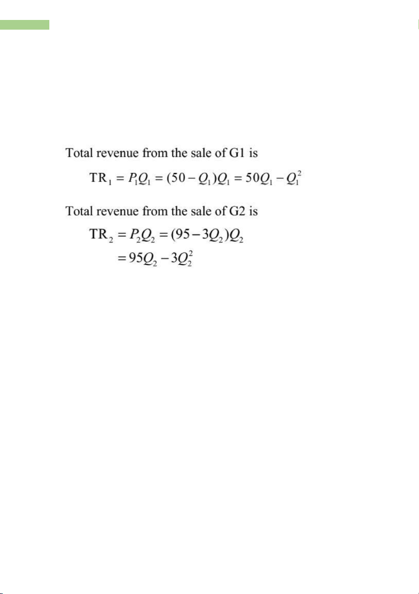
Example: A firm is a monopolistic producer of two goods G1 and G2. The prices are related
to quantities Q1 and Q2 according to the demand functions: P1 = 50 – Q1
10 TR¯¡NG THANH HOA – MATHEMATICS FOR BUSINESS P2 = 95 – 3Q2 If the total cost function is TC = Q 2 2 1 + 3Q1Q2 +Q2
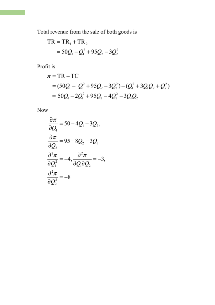
Show that the firm’s profit function is �㔋 = 5 Ā 0 2 2
1 2 2Ā1 2 95Ā2 2 4Ā2 2 3Ā1Ā2
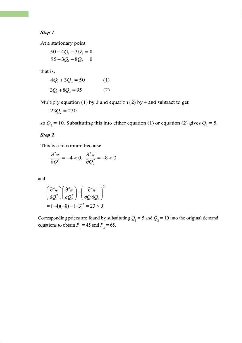
Hence find the values of Q1 and Q2 which maximise �㔋 and deduce the corresponding prices.
11 TR¯¡NG THANH HOA – MATHEMATICS FOR BUSINESS
12 TR¯¡NG THANH HOA – MATHEMATICS FOR BUSINESS Example:
13 TR¯¡NG THANH HOA – MATHEMATICS FOR BUSINESS
14 TR¯¡NG THANH HOA – MATHEMATICS FOR BUSINESS
15 TR¯¡NG THANH HOA – MATHEMATICS FOR BUSINESS
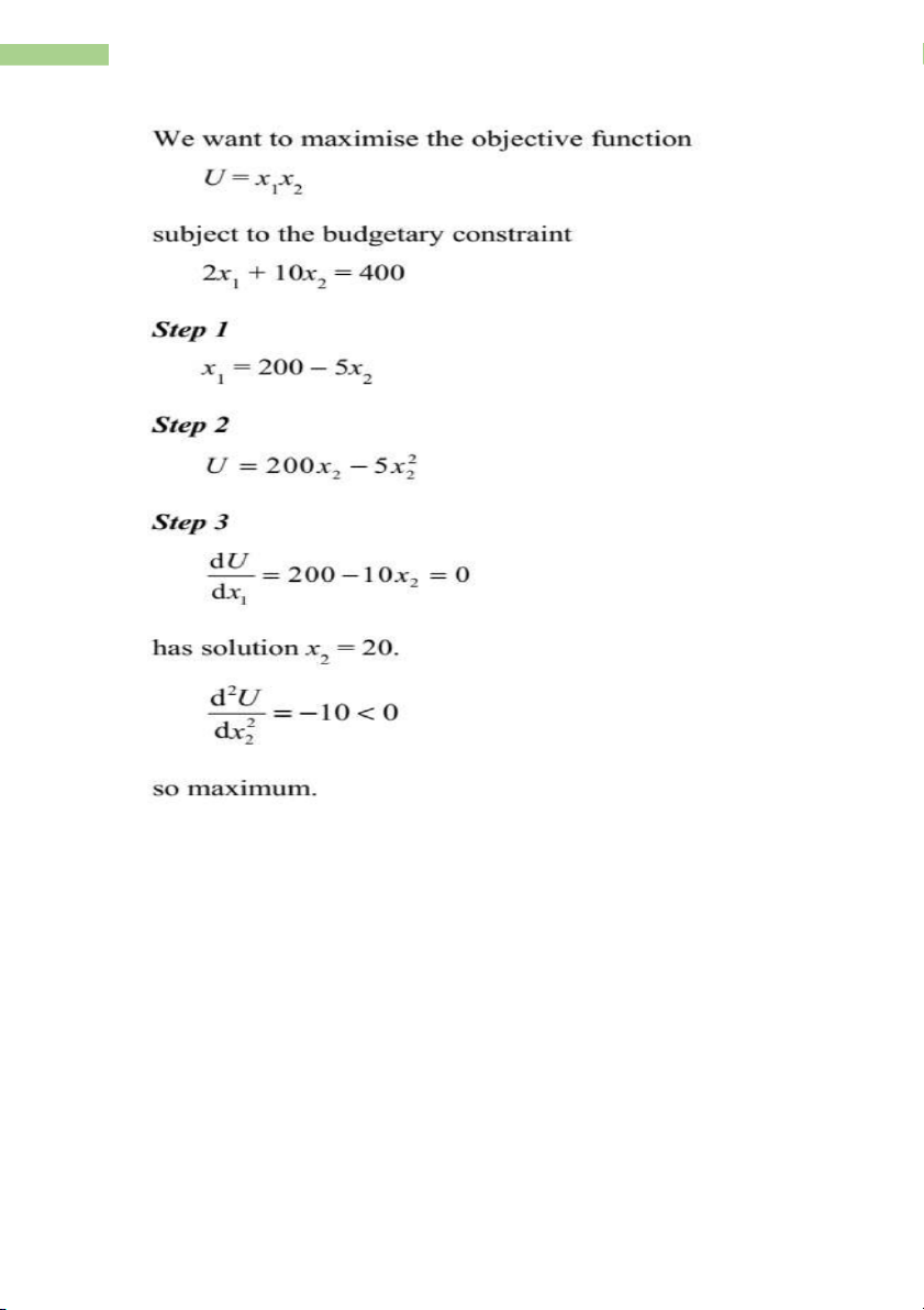
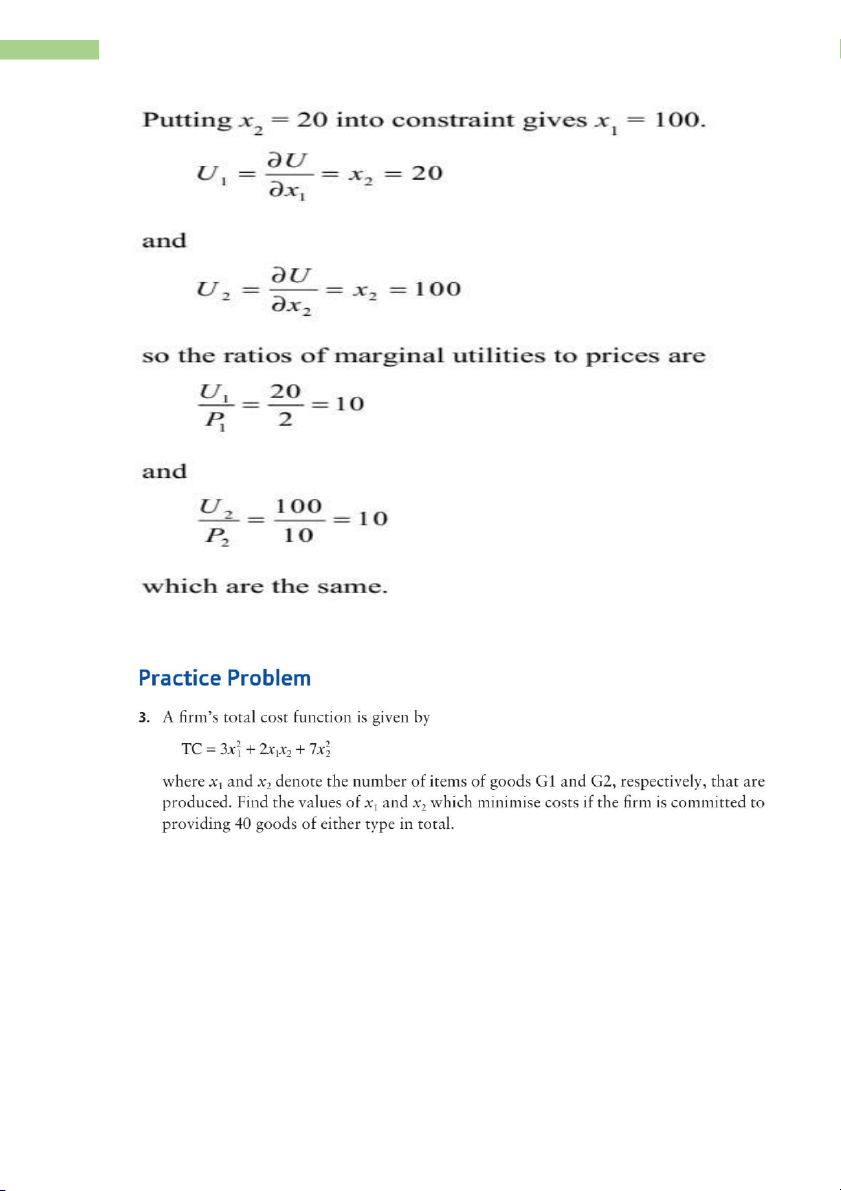
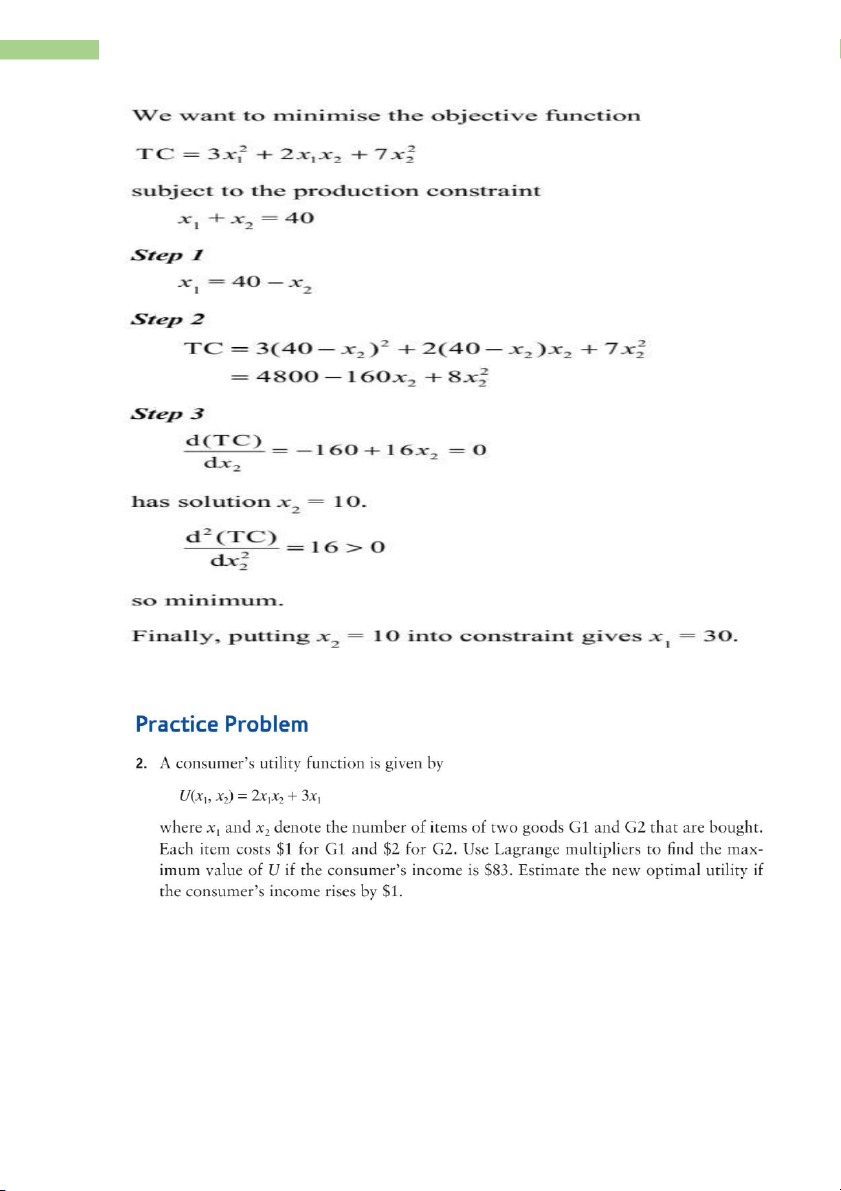
5.2. Finding max/min under constraint
5.2.1. The substitution method
- Optimise y = f(x,z) subject to M = g(x,z).
- Step 1: Use the constraint to express z in terms of x.
- Step 2: Substitute expression for z into the objective function.
- Step 3: Find the value of x that maximises or minimises the objective function.
- Step 4: Substitute this value into constraint to find corresponding value of z.
- Step 5: Substitute values for x and z to find optimal value of y (if required). Example:
16 TR¯¡NG THANH HOA – MATHEMATICS FOR BUSINESS
17 TR¯¡NG THANH HOA – MATHEMATICS FOR BUSINESS
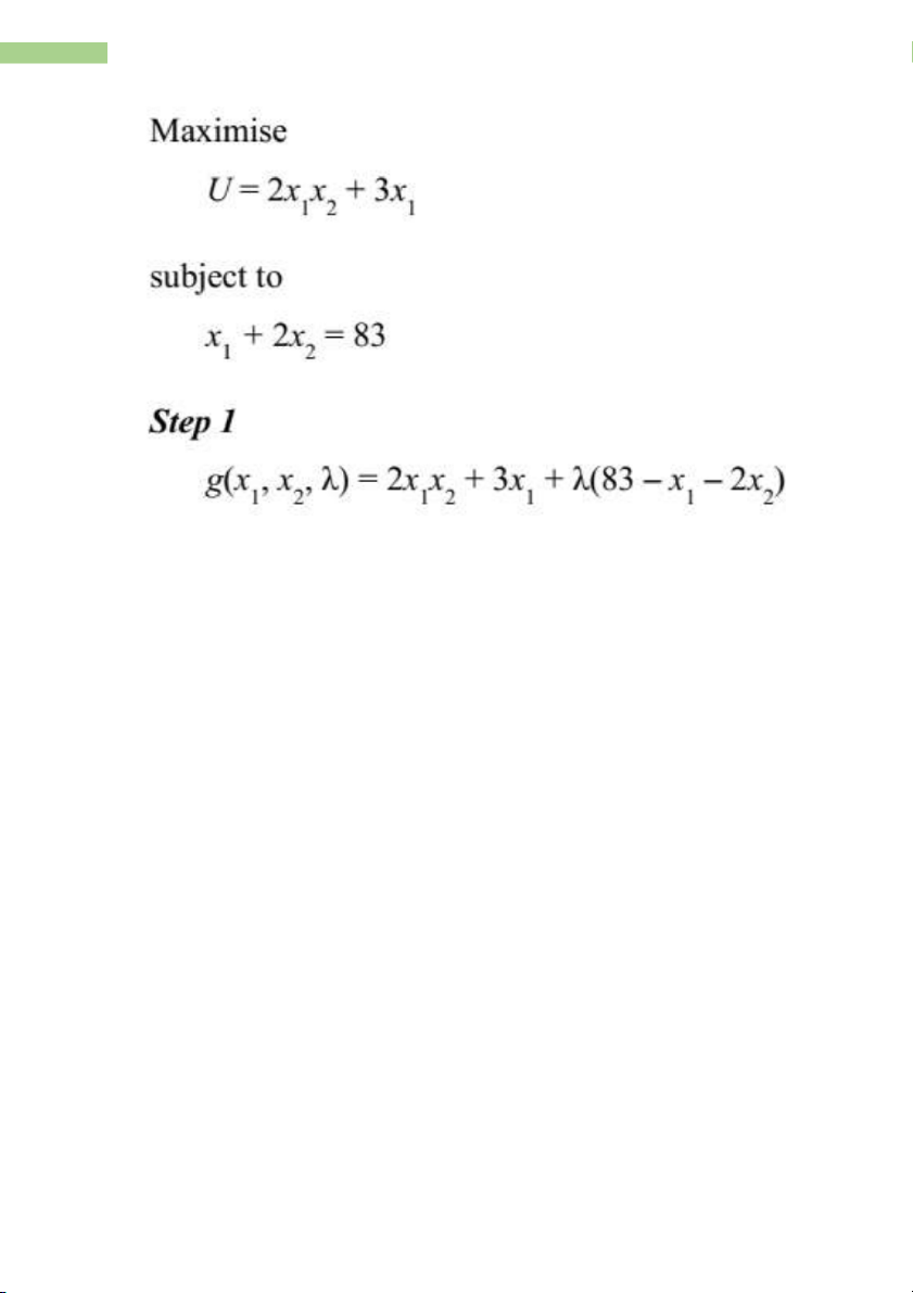
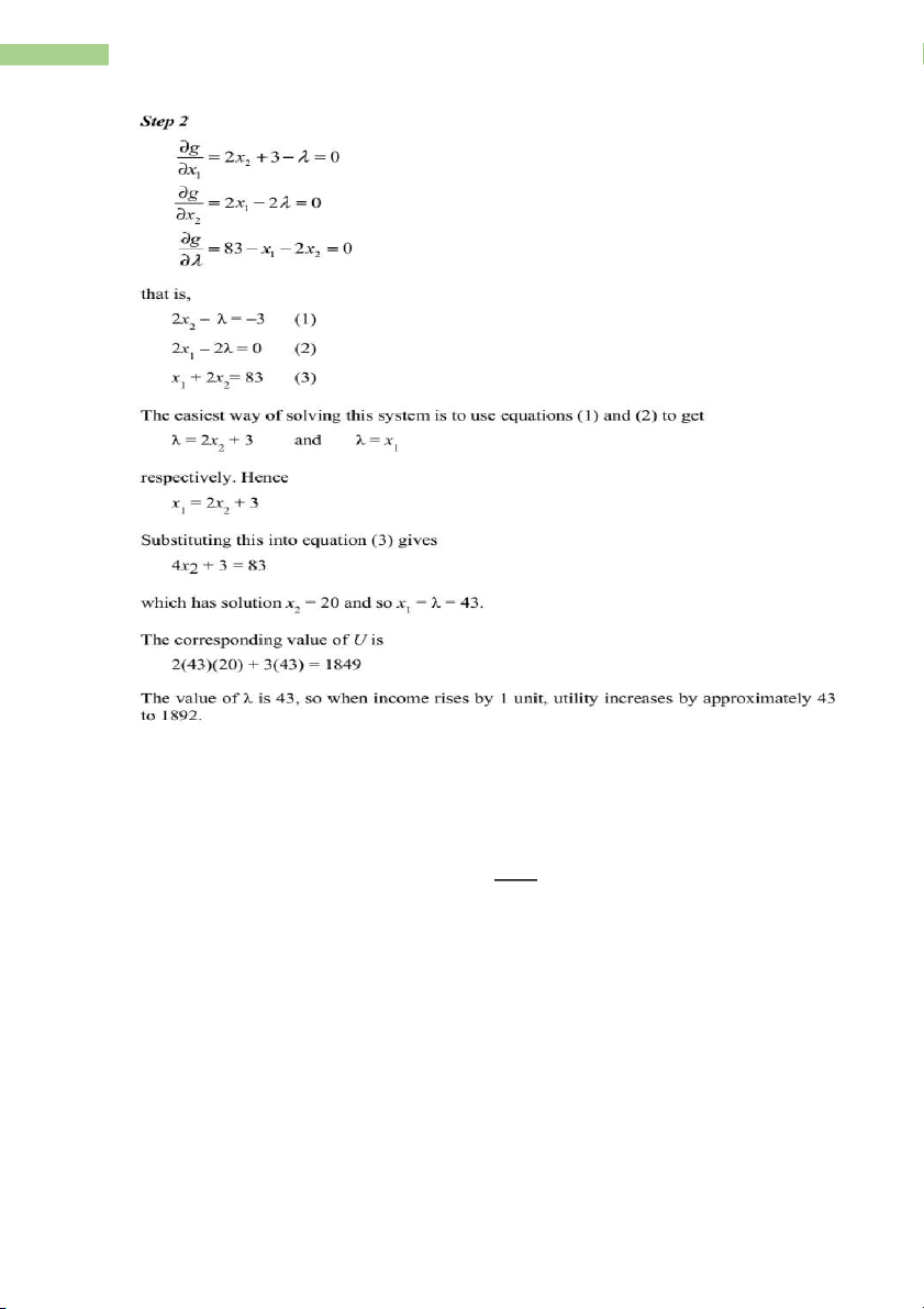
5.2.2. The Lagrange Multiplier Method
- Optimise y = f(x,z) subject to M = g(x,z).
- Step 1: Define a new function:
Ā = Ą(ý, ÿ) + �㔆(ā 2 ą(ý, ÿ))
- Step 2: Find all first order partial derivatives.
- Step 3: Solve the system of equations: �㔕Ā �㔕Ā �㔕Ā �㔕ý = 0, �㔕ÿ = 0, �㔕�㔆 = 0
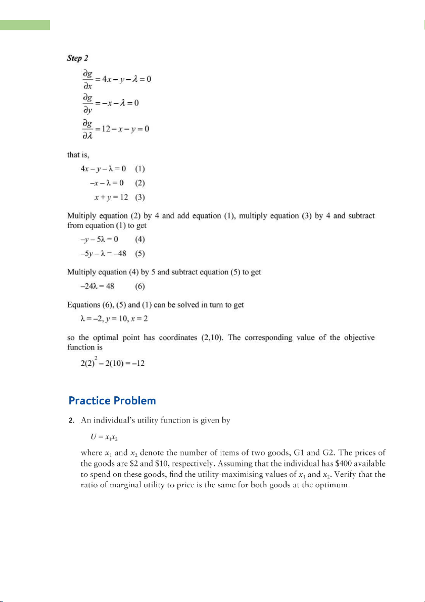
- Step 4: Substitute values for x and z to find optimal value of y (if required). Example:
18 TR¯¡NG THANH HOA – MATHEMATICS FOR BUSINESS
19 TR¯¡NG THANH HOA – MATHEMATICS FOR BUSINESS Example:
20 TR¯¡NG THANH HOA – MATHEMATICS FOR BUSINESS
21 TR¯¡NG THANH HOA – MATHEMATICS FOR BUSINESS Example:
22 TR¯¡NG THANH HOA – MATHEMATICS FOR BUSINESS Example:
23 TR¯¡NG THANH HOA – MATHEMATICS FOR BUSINESS
24 TR¯¡NG THANH HOA – MATHEMATICS FOR BUSINESS CHAPTER 6: INTEGRATION
1. RULES FOR INTEGRATION - Rule 1: 1
Ă(ý) = ∫ ý�㕛. Ăý =ÿ +1ý�㕛+1 +ā - Rule 2:
Ă(ý) = ∫ ÿĄ(ý)Ăý = ÿ ∫ Ą(ý)Ăý - Rule 3:
Ă(ý) = ∫[Ą(ý) ± ą(ý)]Ăý = ∫ Ą(ý)Ăý ± ∫ ą(ý)Ăý
25 TR¯¡NG THANH HOA – MATHEMATICS FOR BUSINESS
2. APPLICATION I: REVENUE, COSTS AND PROFIT
- Calculating marginal functions: Ă(ăā) āā = ĂĀ Ă(ăÿ) āÿ = ĂĀ
- Given MR and MC, use integration to find TR and TC: ăā(Ā) = ∫ āā(Ā)ĂĀ ăÿ(Ā) = ∫ āÿ(Ā)ĂĀ Example:
(a) A firm’s marginal cost function is MC = 2
Find an expression for the total cost function if the fixed costs are 500. Hence find the total cost of producing 40 goods.
(b) The marginal revenue function of a monopolistic producer is MR = 100 – 6Q
Find the total revenue function and deduce the corresponding demand function. (a)
ăÿ = ∫ 2ĂĀ = 2Ā + ā
Fixed costs are 500, so c = 500. Hence TC = 2Q + 500
Put Q = 40 to get TC = 580 (b)
ăā = ∫(100 2 6Ā)ĂĀ = 10 Ā 0 2 2Ā2 + ā
Revenue is zero when Q = 0, so c = 0. Hence ăā = 100Ā 2 3Ā2
26 TR¯¡NG THANH HOA – MATHEMATICS FOR BUSINESS ăā 100Ā 2 3Ā2 ÿ = Ā = Ā = 100 2 3Ā
So demand equation is P = 100 – 3Q.
3. DEFINITE INTEGRATION Ā
∫ Ą(ý)Ăý = [Ă(ý)] Āÿ = Ă(Ā) 2 Ă(ÿ) ÿ
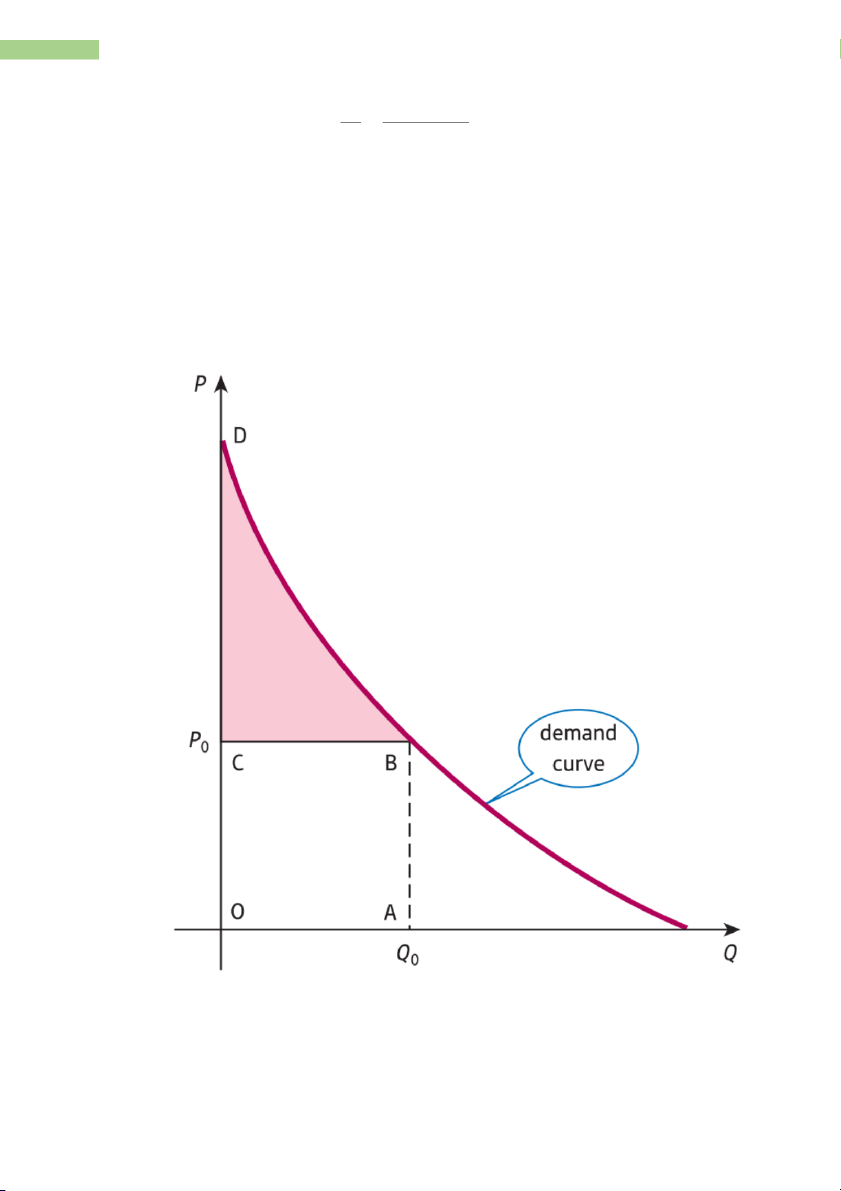
4. APPLICATION II: CONSUMER AND PRODUCER SURPLUS
- Consumer surplus: amount consumers are willing to pay for a good in excess of actual price charged.
27 TR¯¡NG THANH HOA – MATHEMATICS FOR BUSINESS Ā1 ÿĂ = ∫ Ā(Ā)ĂĀ2 ÿ1Ā1 0
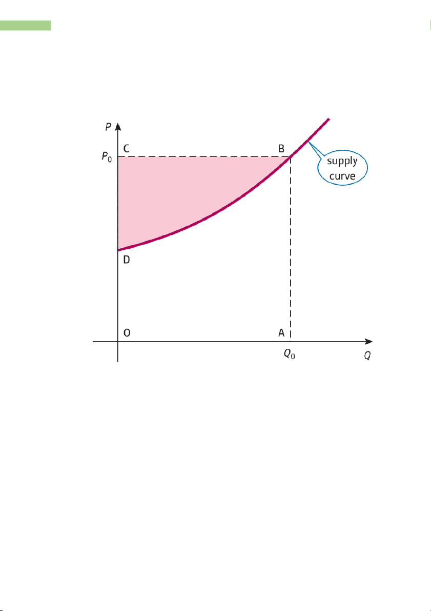
- Producer surplus: amount in below actual price charged that producers are willing to aupply the good. Ā1
ÿĂ = ÿ1Ā1 2 ∫ Ă(Ā)ĂĀ 0
Example: Find the consumer’s surplus at Q = 8 for the demand function: ÿ = 100 2 Ā2
Substitute Q = 8 to get ÿ = 100 2 82 = 36 8
ÿĂ = ∫ (100 2 Ā2)ĂĀ 2 8 ý 36 0
28 TR¯¡NG THANH HOA – MATHEMATICS FOR BUSINESS 1 8 = [10 Ā 0 2 2 288 = 341.33 3 Ā3] 0
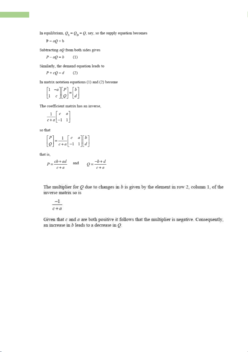
Example: Given the demand equation P = 50 − 2QD and supply equation P = 10 + 2QS Calculate (a) the consumer’s surplus (b) the producer’s surplus assuming pure competition.
In equilibrium, QS = QD = Q, so P = 50 – 2Q P = 10 + 2Q Hence,
50 – 2Q = 10 + 2Q
Which has solution Q = 10. The demand equation gives
P = 50 – 2 x 10 = 30 (a) 10
ÿĂ = ∫ (50 2 2Ā)ĂĀ 2 10 ý 30 = 100 0 (b) 10
ÿĂ = 10 ý 30 2 ∫ (10 + 2Ā)ĂĀ = 100 0
5. APPLICATION III: INVESTMENT FLOW
- Net investment, I, is defined to be the rate of change of capital stock, K, so that where Ăÿ �㔼 = Ăā
I (t) denotes the flow of money, measured in dollars per year.
K (t) is the amount of capital accumulated at time t as a result of this investment flow and is measured in dollars.
29 TR¯¡NG THANH HOA – MATHEMATICS FOR BUSINESS
Hence, given the net investment function, we integrate to find the capital stock. In particular,
to calculate the capital formation during the time period from t = t1 to t = t2 we evaluate the definite integral: �㕡2 ∫ �㔼(ā)Ăā �㕡1
Example: If the net investment function is given by �㔼(ā) = 800ā1/3 Calculate
(a) the capital formation from the end of the first year to the end of the eighth year.
(b) the number of years required before the capital stock exceeds $48 600. (a) 8 3 48
∫ 800ā1/3Ăā= 800 [ 3] = 9000 1 4 ā 1 (b) �㕇 3 4 � 㕇 ∫ 800ā1/3Ăā= 800 [ 3] = 600ă4/3 0 4 ā 0 We need to solve 600ă4/3 = 48,600 That is, ă4/3 = 81 So ă = 813/4 = 27
6. APPLICATION IV: DISCOUNTING
- If the fund is to provide a continuous revenue stream for n years at an annual rate of S
dollars per year then the present value can be found by evaluating the definite integral. �㕛 ÿ = ∫ Ăă2�㕟�㕡/100 Ăā 0
Example: Calculate the present value of a continuous revenue stream for 10 years at a constant
rate of $5000 per year if the discount rate is 6%.
30 TR¯¡NG THANH HOA – MATHEMATICS FOR BUSINESS 10 ÿ = ∫ 5000ă20.06�㕡Ăā = 37,599.03 0 CHAPTER 7: MATRICES I. MATRICES
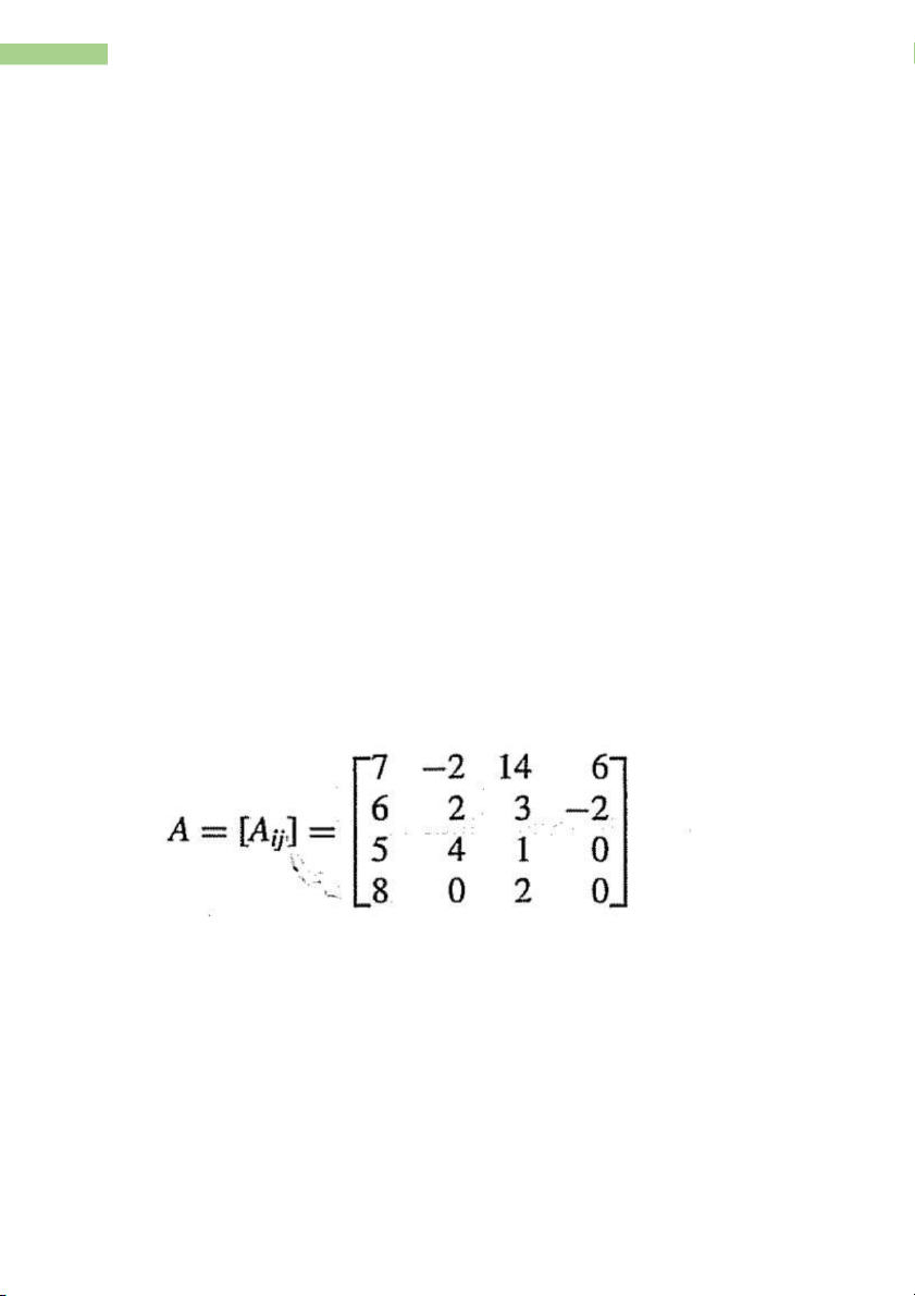
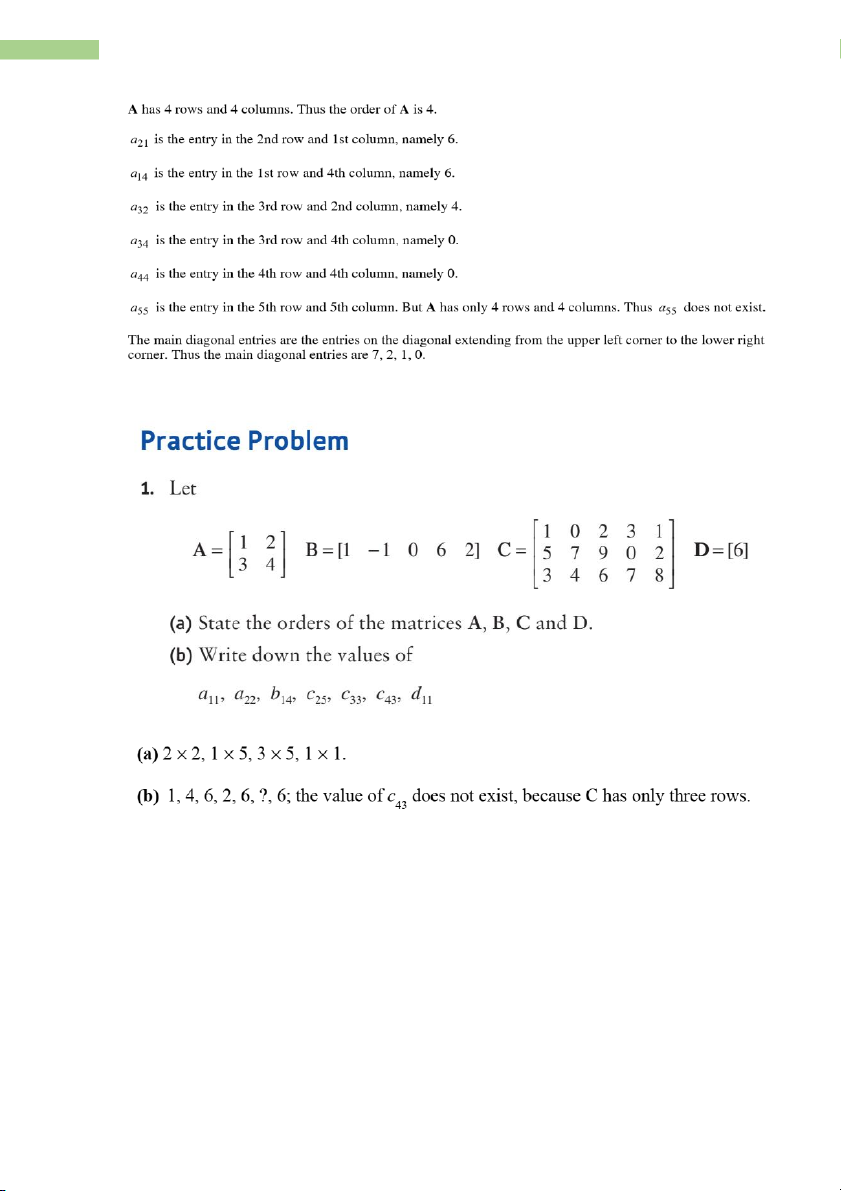
- A matrix consisting of m horizontal rows and n vertical columns is called an m×n matrix or a matrix of size m×n. ùa11 a ... 12 a1 ù n ú ú úa21 a ... 12 a2n ú ú . . ... . ú ú ú ú . . ... . ú ú . . ... . ú ú ú úûa 1 a ... 2 a m m mn ú û
- For the entry aij, we call i the row subscript and j the column subscript. Example: What is the order of A? Find the following entries. A21, A42, A32, A34, A44, A55
What are the third row entries?
31 TR¯¡NG THANH HOA – MATHEMATICS FOR BUSINESS Example: II. MATRIX OPERATIONS
1. Equality of Matrices
- Matrices A = [aij ] and B = [bij] are equal if they have the same size and aij = bij for each i and j.
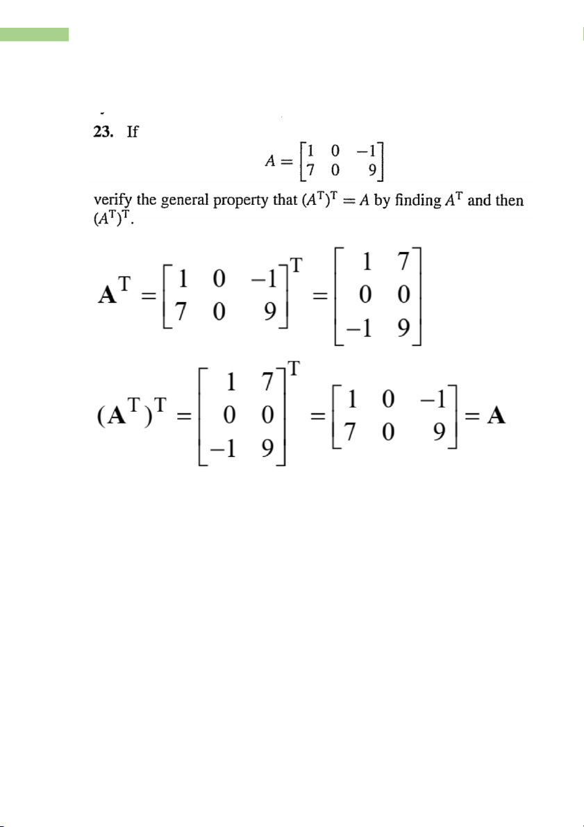
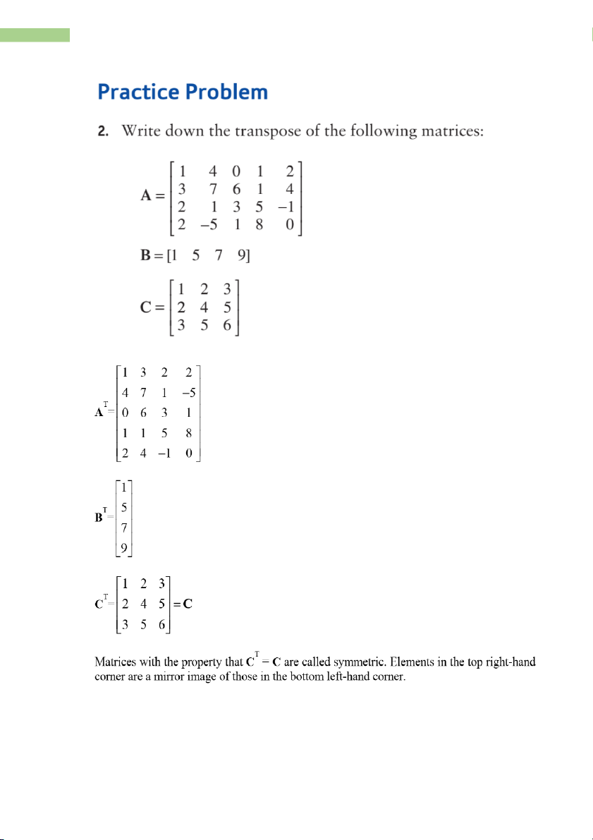
2. Transpose of a matrix
32 TR¯¡NG THANH HOA – MATHEMATICS FOR BUSINESS
- A transpose matrix is denoted by AT. Example: Example:
33 TR¯¡NG THANH HOA – MATHEMATICS FOR BUSINESS
34 TR¯¡NG THANH HOA – MATHEMATICS FOR BUSINESS
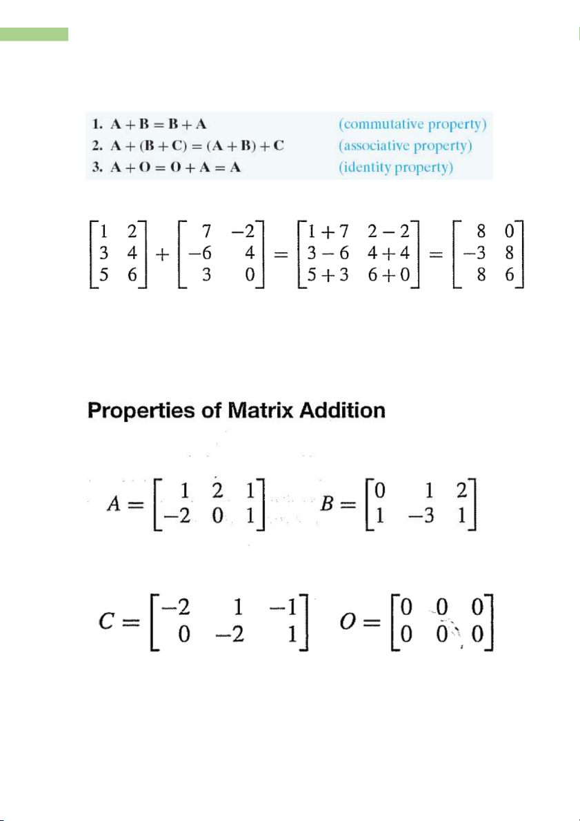
3. Matrix addition
- Sum A + B is the m × n matrix obtained by adding corresponding entries of A and B. Example: ù1 2ù ù2ù + ú ú ú ú
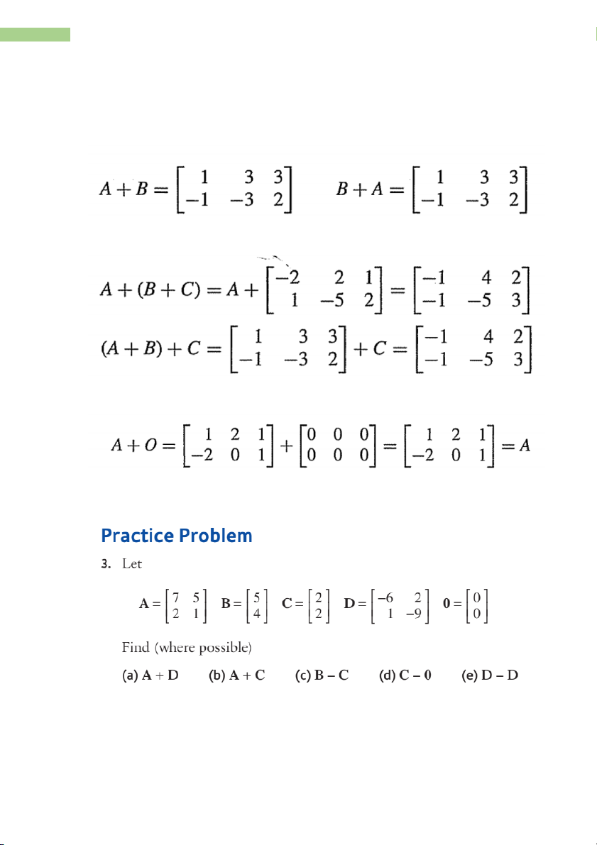
û3 4û û1û is impossible as matrices are not of the same size. Example: a. Show that A + B = B + A
35 TR¯¡NG THANH HOA – MATHEMATICS FOR BUSINESS
b. Show that A + (B + C) = (A + B) + C c. Show that A + O = A a. b. c. Example:
36 TR¯¡NG THANH HOA – MATHEMATICS FOR BUSINESS
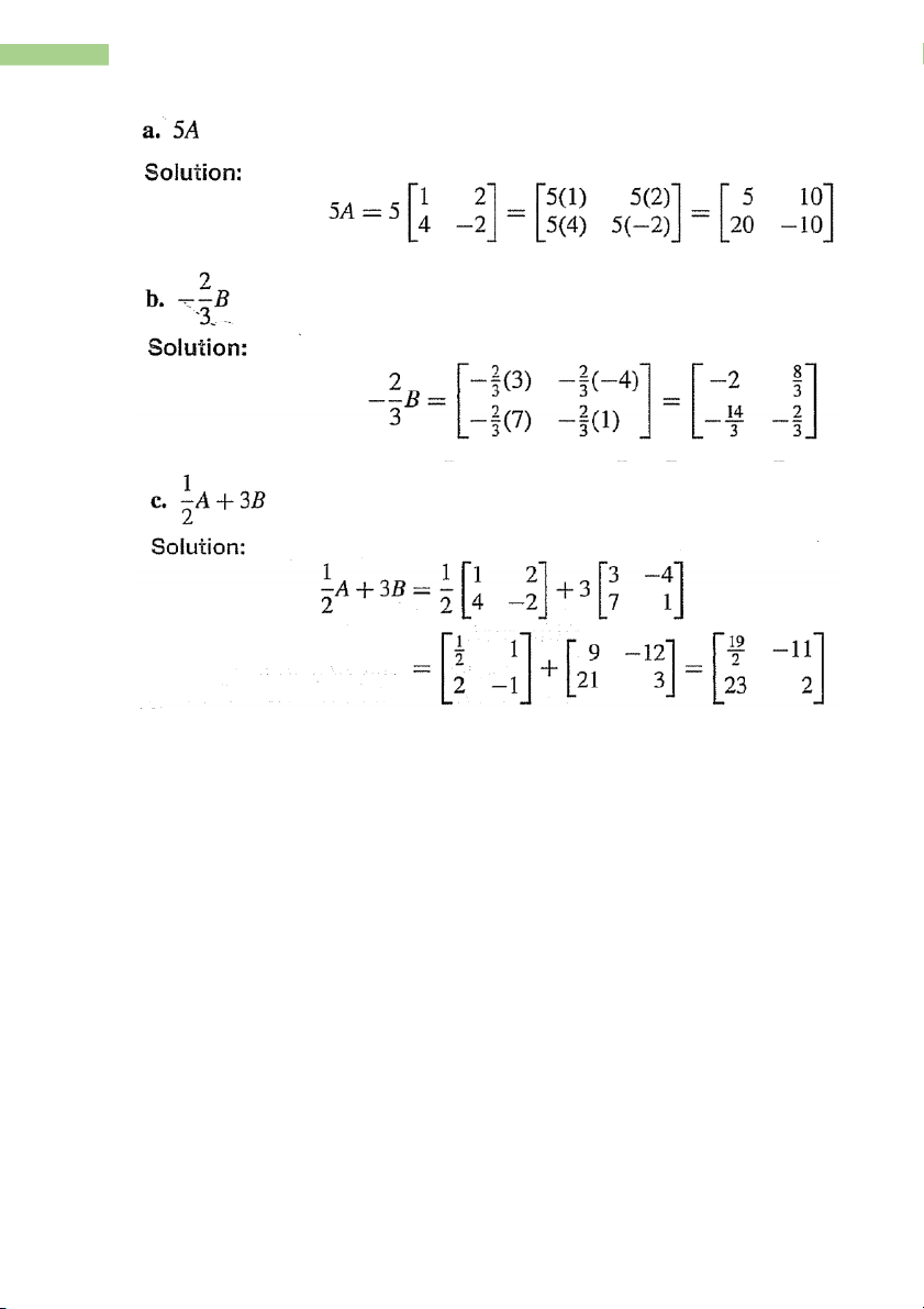
4. Scalar multiplication
5. Subtraction of Matrices
− A = (− )1 A Example:
37 TR¯¡NG THANH HOA – MATHEMATICS FOR BUSINESS Example: ù 2 6ù ù6 − ù 2 ù 2− 6 6 + ù 2 ù− 4 8 ù ú ú ú ú ú ú ú ú − 4 1 − 4 1 = − 4− 4 − 1 1 = ú ú ú ú ú ú ú− 8 0 ú ú 3 2ú ú0 3 ú ú 3 + 0 2 − 3ú ú 3 − ú û û û û û û û û 1
38 TR¯¡NG THANH HOA – MATHEMATICS FOR BUSINESS Example:
39 TR¯¡NG THANH HOA – MATHEMATICS FOR BUSINESS
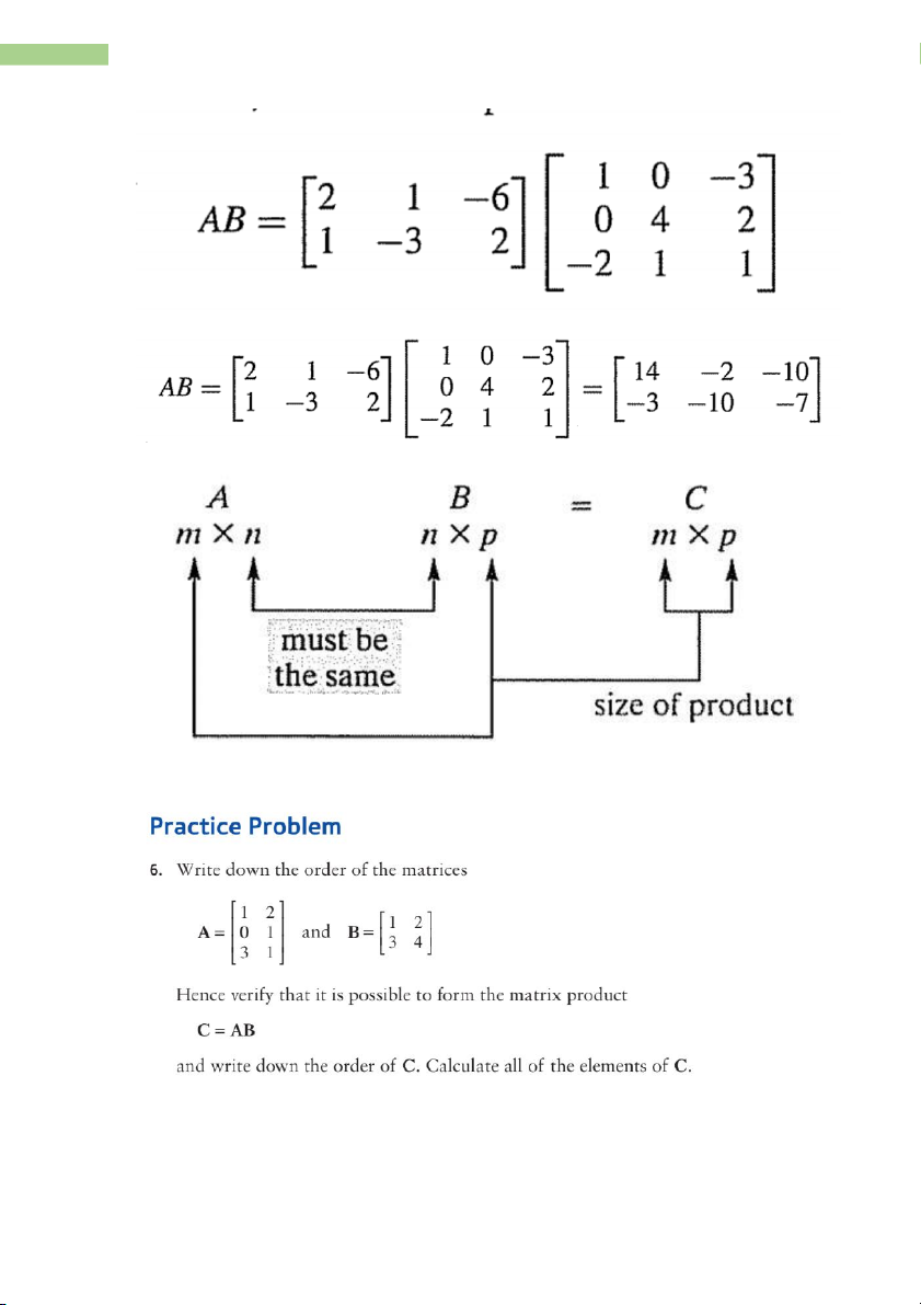
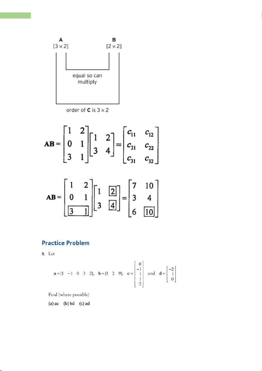
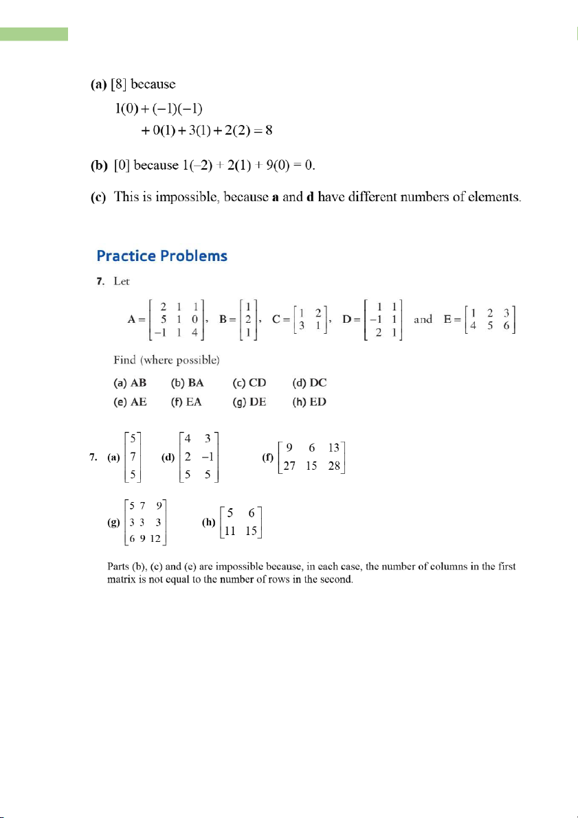
6. Matrix Multiplication
- AB is the m× m
p atrix C whose entry cij is given by: n c = a b = a b 1 1 a + b 2 +... 2 + a b ij ik kj i j i j in nj k =1 Example:
40 TR¯¡NG THANH HOA – MATHEMATICS FOR BUSINESS Example:
41 TR¯¡NG THANH HOA – MATHEMATICS FOR BUSINESS Example:
42 TR¯¡NG THANH HOA – MATHEMATICS FOR BUSINESS Example:
43 TR¯¡NG THANH HOA – MATHEMATICS FOR BUSINESS
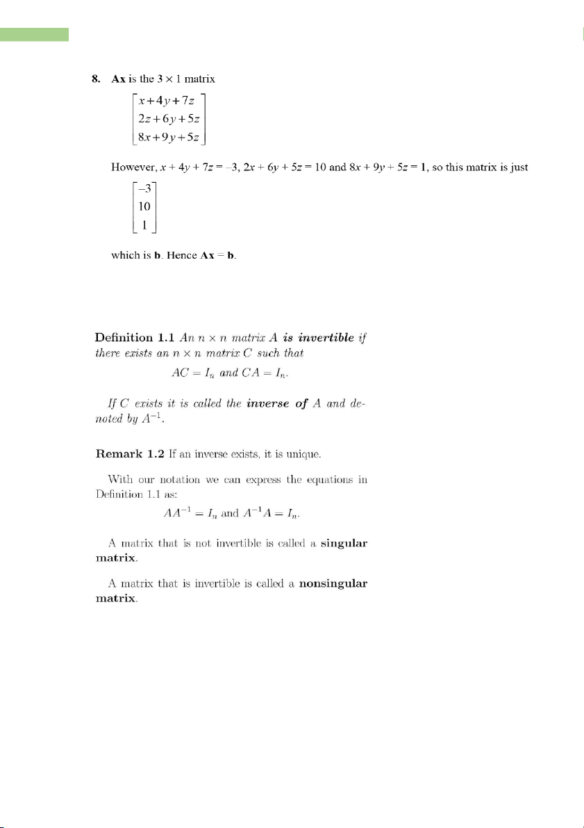
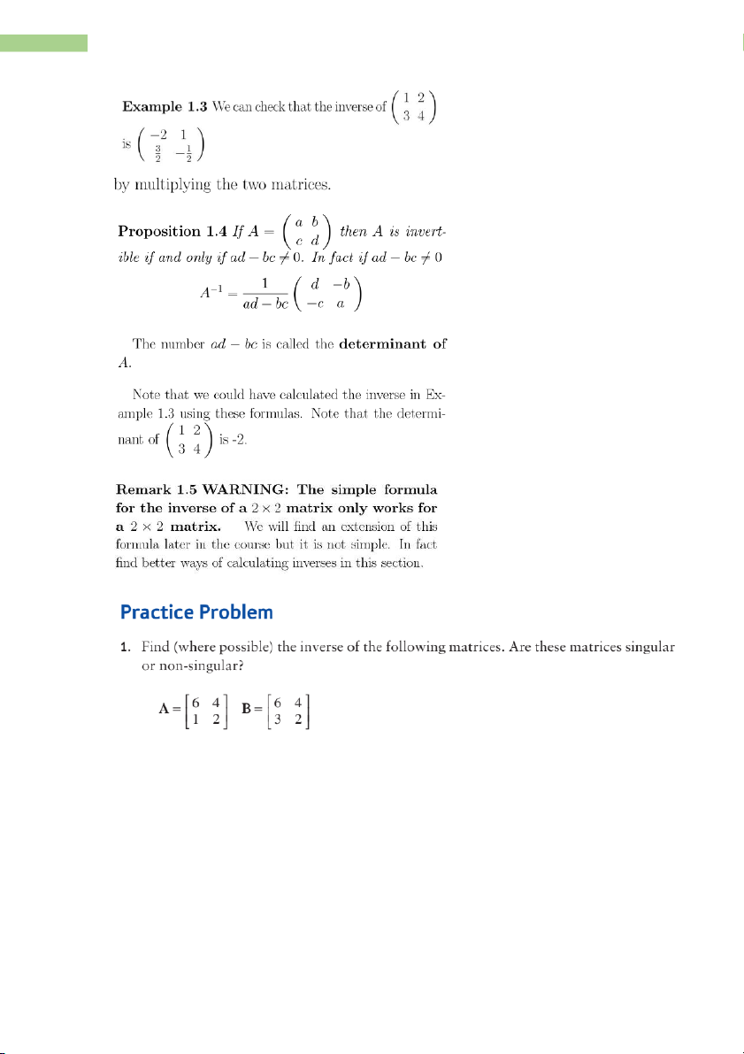
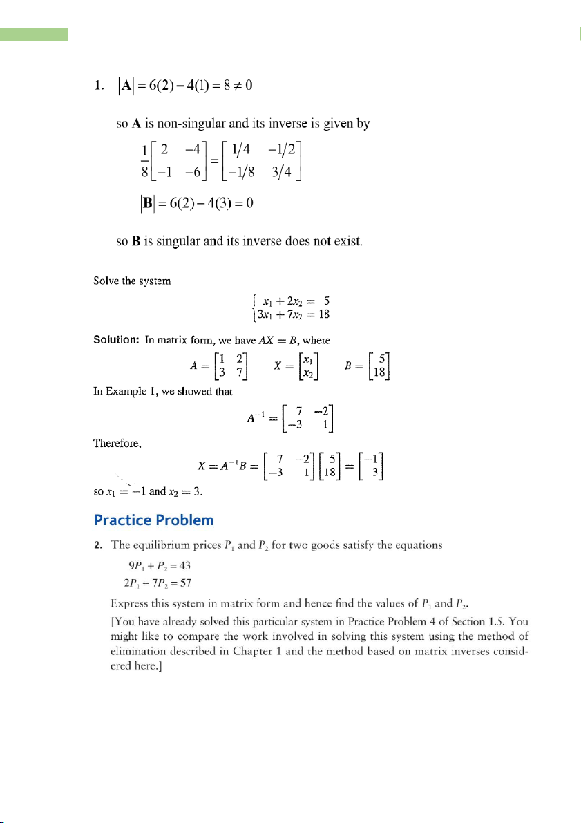
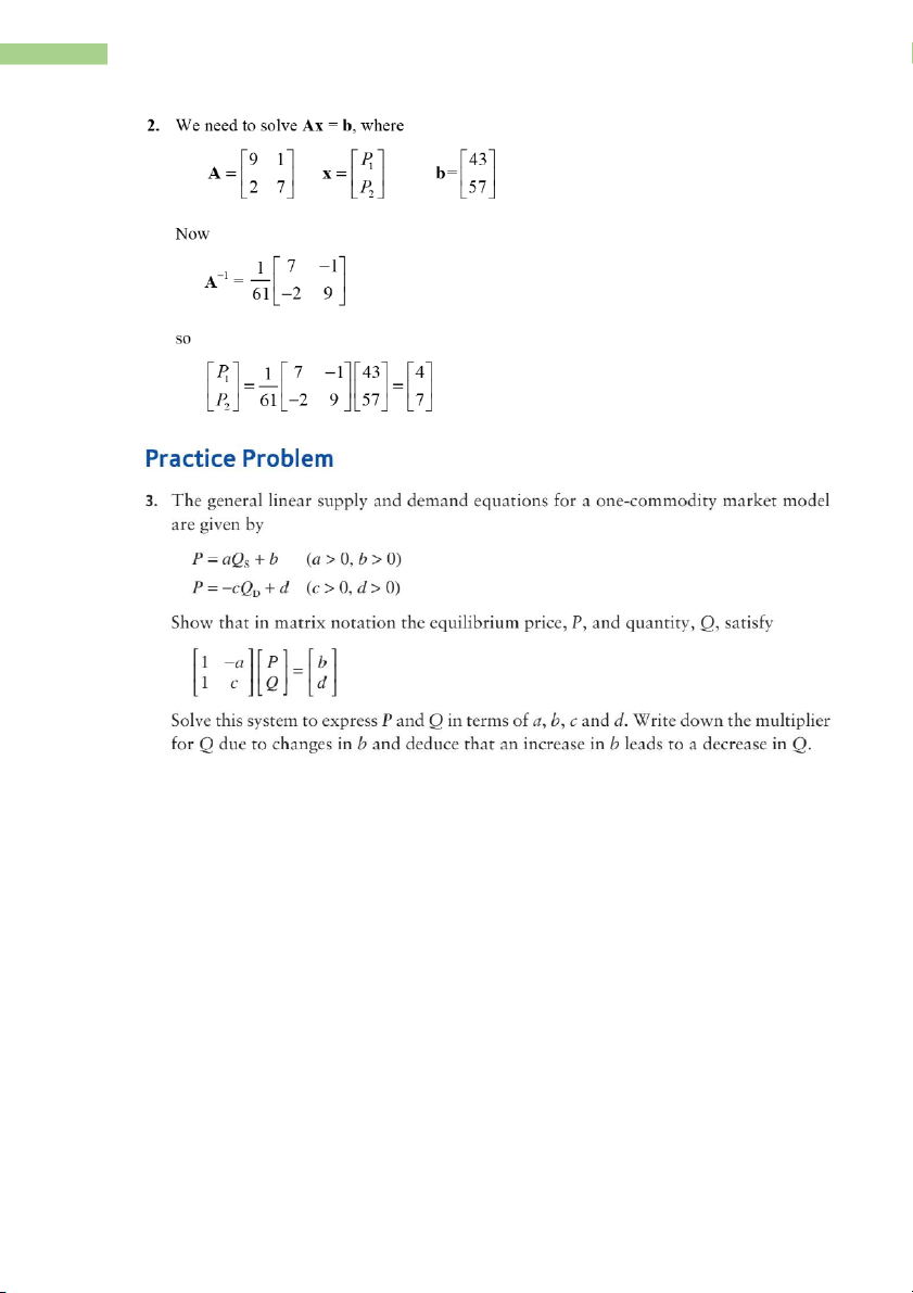
44 TR¯¡NG THANH HOA – MATHEMATICS FOR BUSINESS III. MATRIX INVERSION 1. Matrix 2x2
45 TR¯¡NG THANH HOA – MATHEMATICS FOR BUSINESS
46 TR¯¡NG THANH HOA – MATHEMATICS FOR BUSINESS
47 TR¯¡NG THANH HOA – MATHEMATICS FOR BUSINESS
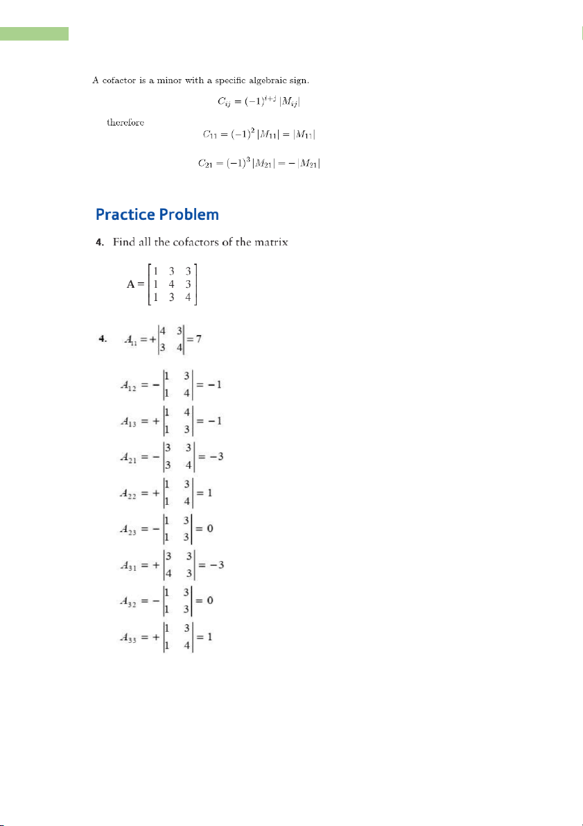
48 TR¯¡NG THANH HOA – MATHEMATICS FOR BUSINESS 2. Matrix 3x3 2.1. Cofactors
49 TR¯¡NG THANH HOA – MATHEMATICS FOR BUSINESS Example:
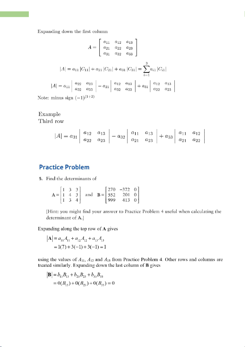
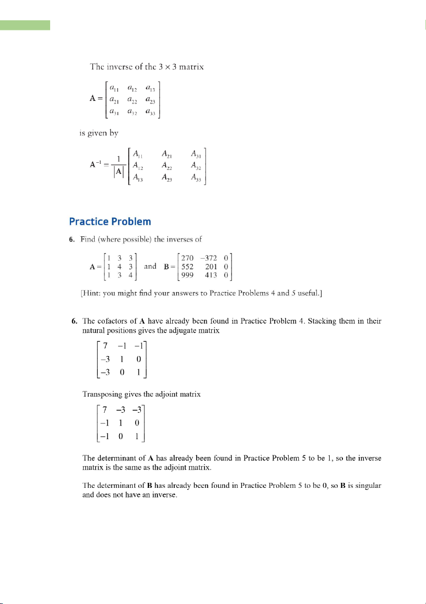
2.2. The determinant and inverse of 3x3 matrix
50 TR¯¡NG THANH HOA – MATHEMATICS FOR BUSINESS Example:
51 TR¯¡NG THANH HOA – MATHEMATICS FOR BUSINESS Example:
52 TR¯¡NG THANH HOA – MATHEMATICS FOR BUSINESS Example: IV. CRAMER’S RULE
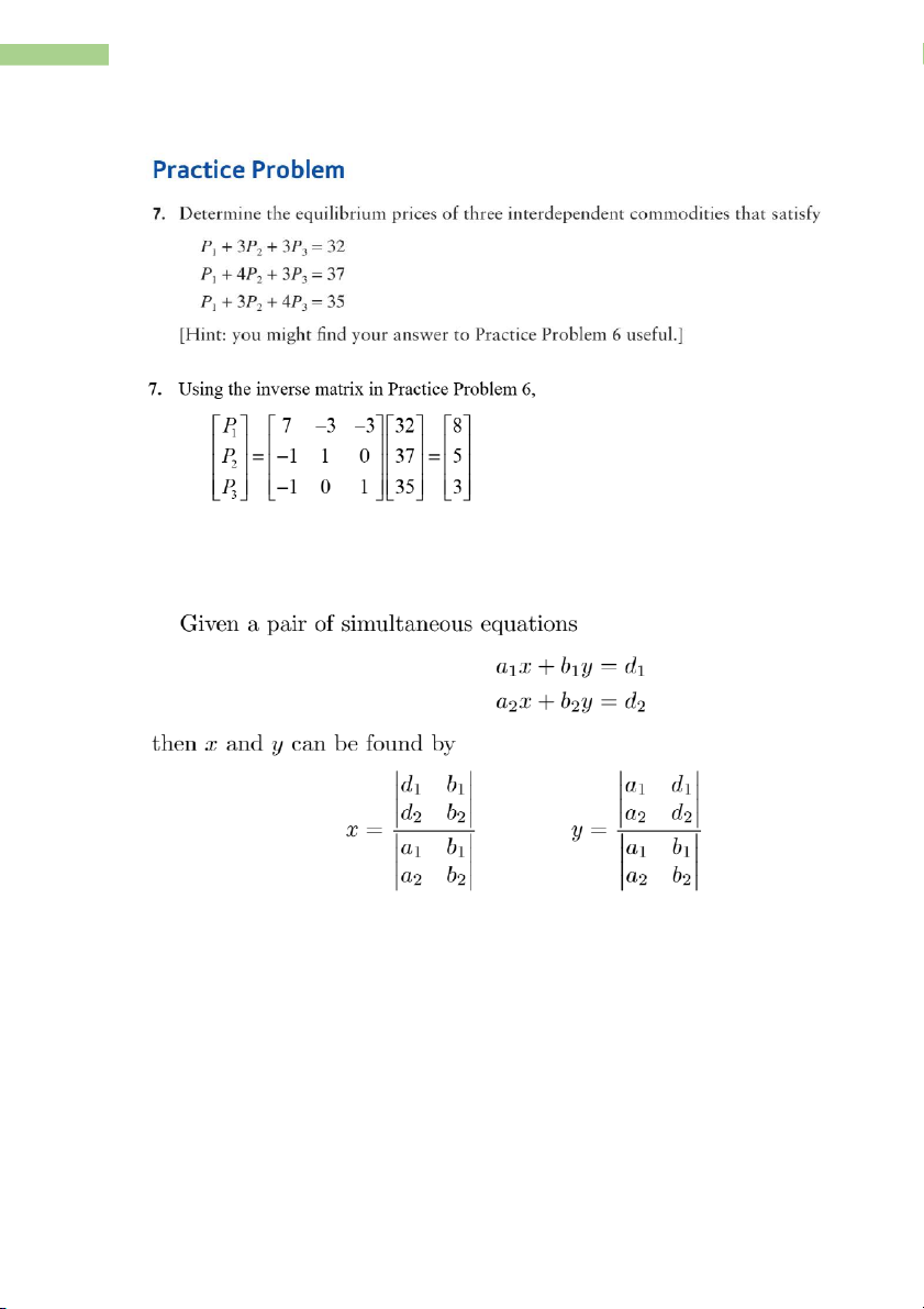
1. Cramer’s Rule for 2 equations
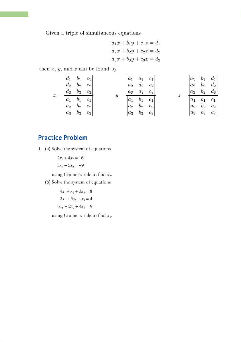
2. Cramer’s Rule for 3 equations
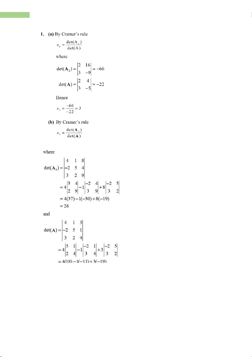
53 TR¯¡NG THANH HOA – MATHEMATICS FOR BUSINESS Example:
54 TR¯¡NG THANH HOA – MATHEMATICS FOR BUSINESS
55 TR¯¡NG THANH HOA – MATHEMATICS FOR BUSINESS
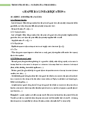
CHAPTER 8: LINEAR PROGRAMMING
- Cách vẽ đ°ờng thẳng y = ax + b:
• Cho x = 0 => y = b => điểm (0, b).
• Cho y = 0 => x = -b/a => m điể (-b/a, 0)
• Nối 2 điểm lại thành đ°ờng thẳng.
- Cách xác định feasible region:
• Chọn 1 điểm nằm ngoài đ°ờng thẳng.
• Thế điểm đó vào ph°¢ng trình.
• Xác định xem điểm đó có thoả mãn bất ph°¢ng trình hay không. Nếu có thì feasible
region chính là vùng chứa điểm đó, nếu không thì feasible region là vùng còn lại
(gạch bỏ vùng chứa điểm đó).
56 TR¯¡NG THANH HOA – MATHEMATICS FOR BUSINESS Example:
57 TR¯¡NG THANH HOA – MATHEMATICS FOR BUSINESS
58 TR¯¡NG THANH HOA – MATHEMATICS FOR BUSINESS Example:
59 TR¯¡NG THANH HOA – MATHEMATICS FOR BUSINESS Example:
60 TR¯¡NG THANH HOA – MATHEMATICS FOR BUSINESS Example:
61 TR¯¡NG THANH HOA – MATHEMATICS FOR BUSINESS
62 TR¯¡NG THANH HOA – MATHEMATICS FOR BUSINESS Example: Example:
63 TR¯¡NG THANH HOA – MATHEMATICS FOR BUSINESS
64 TR¯¡NG THANH HOA – MATHEMATICS FOR BUSINESS Example:
65 TR¯¡NG THANH HOA – MATHEMATICS FOR BUSINESS
Example: An electronics firm decides to launch two models of a tablet, TAB1 and TAB2. The
cost of making each device of type TAB1 is $120 and the cost for TAB2 is $160. The firm
recognises that this is a risky venture so decides to limit the total weekly production costs to
$4000. Also, due to a shortage of skilled labour, the total number of tablets that the firm can
produce in a week is at most 30. The profit made on each device is $60 for TAB1 and $70 for
TAB2. How should the firm arrange production to maximise profit?
66 TR¯¡NG THANH HOA – MATHEMATICS FOR BUSINESS
Example: A publisher decides to use one section of its plant to produce two textbooks called
Microeconomics and Macroeconomics . The profit made on each copy is $12 for
Microeconomics and $18 for Macroeconomics. Each copy of Microeconomics requires 12
minutes for printing and 18 minutes for binding. The corresponding figures for
Macroeconomics are 15 and 9 minutes, respectively. There are 10 hours available for printing
and 10.5 hours available for binding. How many of each should be produced to maximise profit?
67 TR¯¡NG THANH HOA – MATHEMATICS FOR BUSINESS