Fuzzy PID Control of a Five DOF Robot Arm: A Comprehensive Study | Môn Công nghệ kỹ thuật cơ điện tử - Đại học Sư phạm Kỹ thuật Thành phố Hồ Chí Minh

lOMoAR cPSD| 58675420 299
Journal of Intelligent and Robotic Systems 40: 299–320, 2004.
© 2004 Kluwer Academic Publishers. Printed in the Netherlands.
Fuzzy PID Control of a Five DOF Robot Arm G. M. KHOURY
Saint-Joseph University, ESIB, Sciences and Technologies Campus, Mar Roukoz, Mkalles, Lebanon M. SAAD
University of Quebec, ETS, 1100 Notre-Dame Street West, Montreal, Quebec, Canada H. Y. KANAAN and C. ASMAR
Saint-Joseph University, ESIB, Sciences and Technologies Campus, Mar Roukoz, Mkalles, Lebanon
(Received: 20 June 2003; in final form: 15 March 2004)
Abstract. This paper studies the application of fuzzy logic control on a five degrees of freedom
(DOF) robot arm, the Maker 100 of U.S. Robots. The elaboration of the fuzzy control laws is based
on two structures of coupled rules fuzzy PID controllers. The fuzzy PID controllers are numerically
simulated and the simulation results confirm the success of the fuzzy PID control in trajectory
tracking problems. Seeking a performance optimization, a systematic study of the choice of tuning
parameters of the controllers is done. The success of the proposed fuzzy control law is again affirmed
by a comparative evaluation with respect to the computed torque control method and the direct
adaptive control method, the last two controls being also numerically implemented using the same
dynamic model of the robot arm.
Key words: five DOF robot arm, fuzzy control, numerical simulation, PID controllers. 1. Introduction
The use of industrial robots became identifiable as a unique device in the 1960s.
Since then, their field of application evolved from rather simple tasks like welding
and painting to those requiring more precision, such as assembly tasks.
Control theory provides tools for designing and evaluating algorithms to realize
desired motions or force application. The methods of linear control and those of
local linearization and moving linearization are not well suited for the control
problem of robotic arms. This is due to the fact that robotic arms constantly move
among widely separated regions of their workspace such that no linearization valid
for all regions can be found. On the other hand, nonlinear control methods are
progressing nowadays and different classes could be identified [13]: Trialand- lOMoAR cPSD| 58675420 300 G. M. KHOURY ET AL.
Error, Feedback Linearization Control, Robust Control, Adaptive Control, and
Gain-Scheduling. Nonlinear control methods used in robot arms’ applications
should however face the major difficulty resulting from the dynamic modeling of
robots, i.e. the indetermination of their parameters [3]. Preferred methods are those
which reduce or eliminate the undesired effects generated by this indetermination
such as the Feedback Linearization control method [13], the Model-Reference
Adaptive control method [12, 13] and the Self-Tuning method [13]. Another
difficulty in robot arm control is the coupling effects of the coriolis and centrifugial
forces that might be canceled in a single axis mode operation where the joints are
activated sequentially. Existing methods of nonlinear control are also used in
robotics in order to eliminate the above mentioned coupling effect like the
Individual Joint PID control method [3] and the PD-plus-gravity control method [3].
Among the recent nonlinear control methods, fuzzy control methods grab
nowadays the attention of many researchers. In fact, these methods do not require
the knowledge of the dynamic model of the controlled system. This feature
becomes of major importance when dealing with complex nonlinear systems.
Moreover, the dynamic modeling of robot arms shows a dependency on their
mechanical parameters, subject to lifetime modifications (friction factors affected
by the abuse of joints), and on their dynamical parameters that vary with the
performed task (centers of gravity of the links affected by tool’s replacements).
These considerations also give advantage to fuzzy control methods on other
nonlinear methods as a result of their robustness towards perturbations affecting the system.
The first fuzzy logic controller was introduced by Mamdani in 1974 [7]. It is
equivalent to two-input fuzzy PI controllers, where error and change of error were
used as the inputs of the inference system. Mamdani’s work also introduced the
most common and robust fuzzy reasoning method, called Zadeh–Mamdani min–
max gravity reasoning. Different comparative studies, like [5], prove that Zadeh–
Mamdani min–max gravity scheme is the best reasoning scheme if the nonlinearity variation is a main concern.
Although control methods, especially nonlinear control methods, had greatly
evolved, the proportional-integral-derivative (PID) control method is still widely
used in all domains [2]. The success of the PID control is attributed to its simplicity
(in terms of design and tuning) and to its good performance in a wide range of
operating conditions. However, the neccesity of retuning the PID controllers
characterizes their major disadvantage when the controlled plant is subject to
disturbances or when it presents complexities (non-linearities).
The majority of applications of fuzzy control methods during the past two
decades belong to the class of fuzzy PID controllers. These fuzzy controllers can
be classified into three types: the direct action (DA) type in which the inference lOMoAR cPSD| 58675420
FUZZY PID CONTROL OF A FIVE DOF ROBOT ARM 301
system provides the main control action, the gain scheduling (GS) type [18] where
the inference system provides instantaneous adjustments on the gains of a classical
linear PID controller, and a combination of DA and GS types. A comparative study
held in [5] shows that the nonlinear equivalent model of a DA-type fuzzy PID
controller is simpler than that of a GS-type fuzzy PID controller where the
nonlinearity is hard to aquier. As a result, the majority of used fuzzy PID
controllers is of the DA-type.
The main objective of this paper is to study and analyse the adaptation of
existing fuzzy DA PID structures to the trajectory tracking control of a robotic
arm containing high nonlinearities. Performance evaluation of the closed loop
system will focus on the ability of the fuzzy PID structures, in terms of tracking
precision and robustness, to control the arm.
This paper is divided into 7 sections. Section 2 introduces the five degrees of
freedom robot arm Maker 100 and its dynamic model. In Section 3, two structures
of DA fuzzy PID controllers are presented along with their tuning method. Section
4 deals with the integration of the fuzzy structures in the control loop while Section
5 is reserved to the numerical simulation of the control laws and a study of the
results and performances. Section 6 provides a comparative evaluation of the fuzzy
PID control method in respect to other methods of nonlinear control, the computed
torque control method and the direct adaptive control method. Finally, Section 7
discusses the benefits of the studied fuzzy control law and proposes
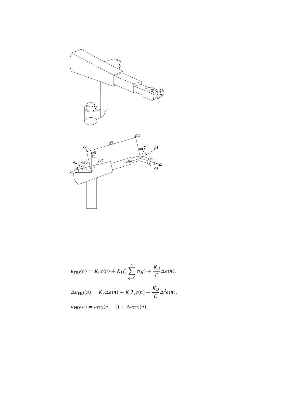
recommendations for a productive continuity in this line of research. 2. The Maker 100
The Maker 100 of U.S. Robots is a five DOF robot arm. All its joints are revolute
joints except the third, which is prismatic. Figure 1 shows the Maker 100 while
Figure 2 shows its structural state variables.
The dynamic model of the Maker 100 is given by Equation (1).
τ = M(q)q¨ + V(q,q)˙ + G(q) + F, (1)
where: τ = [τ1 τ2 τ3 τ4 τ5]T the joint input torque vector, q = [θ1 θ2 d3 θ4 θ5]T the joint
position vector, q˙ = [θ˙1 θ˙2 d˙3 θ˙4 θ˙5]T the joint velocity vector, q¨ = [θ¨1 θ¨2 d¨3 θ¨4
θ¨5]T the joint acceleration vector.
Note that vectors q, q˙ and q¨ are defined in the joint space.
And: M positive definite inertia and mass matrix, V matrix of coriolis and
centrifugal forces, G state varying vector of gravity terms, F state matrix of friction terms. M(q),V(q,q),G(q)˙
and F are given in Appendix A. lOMoAR cPSD| 58675420 302 G. M. KHOURY ET AL. Figure 1. Maker 100.
Figure 2. State variables representation.
3. Fuzzy PID Structures
Refering to [8], the control signal of a linear PID at any given time instance n with
a sampling time Ts can be expressed in its absolute form, expression (2), or in its
incremental form, expression (3). (2) (3) where .
The terms KP, KI, and KD stand for proportional, integral, and derivative gains,
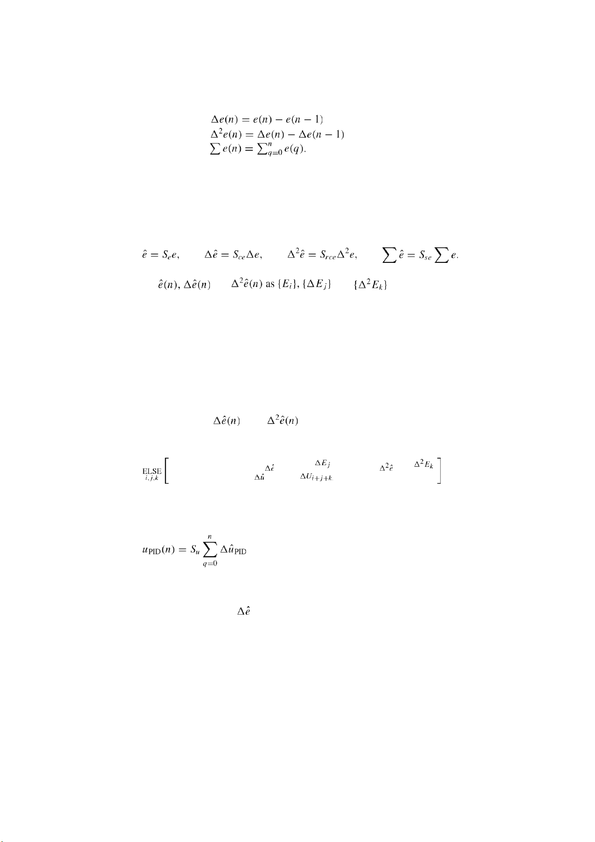
respectively. The error state variables are defined as: lOMoAR cPSD| 58675420
FUZZY PID CONTROL OF A FIVE DOF ROBOT ARM 303 Error e(n) = y(n) − yd(n), Error change , Rate of error change , Sum-of-error
The term y(n) is the feedback response signal, and yd(n) is the desired response or
reference input at the nth sampling instant. In a fuzzy PID controller, the error
terms in (2) or (3) are expressed in a linguistic form and the fuzzy rules are used
to infer a fuzzy control action. Scale factors Sx for each error state variable x are
defined to obtain the normalized error terms, whose values are chosen within the range [−1,1], as:
Finally we define the linguistic variables that correspond to the input scaled variables , and , and respectively, where:
i = 0,1,2,... ,Ne − 1; j = 0,1,2,... ,Nce − 1; k = 0,1,2,... ,Nrce − 1.
Ne, Nce, and Nrce denote the total numbers of fuzzy membership functions assigned
for each of the fuzzy linguistic variables.
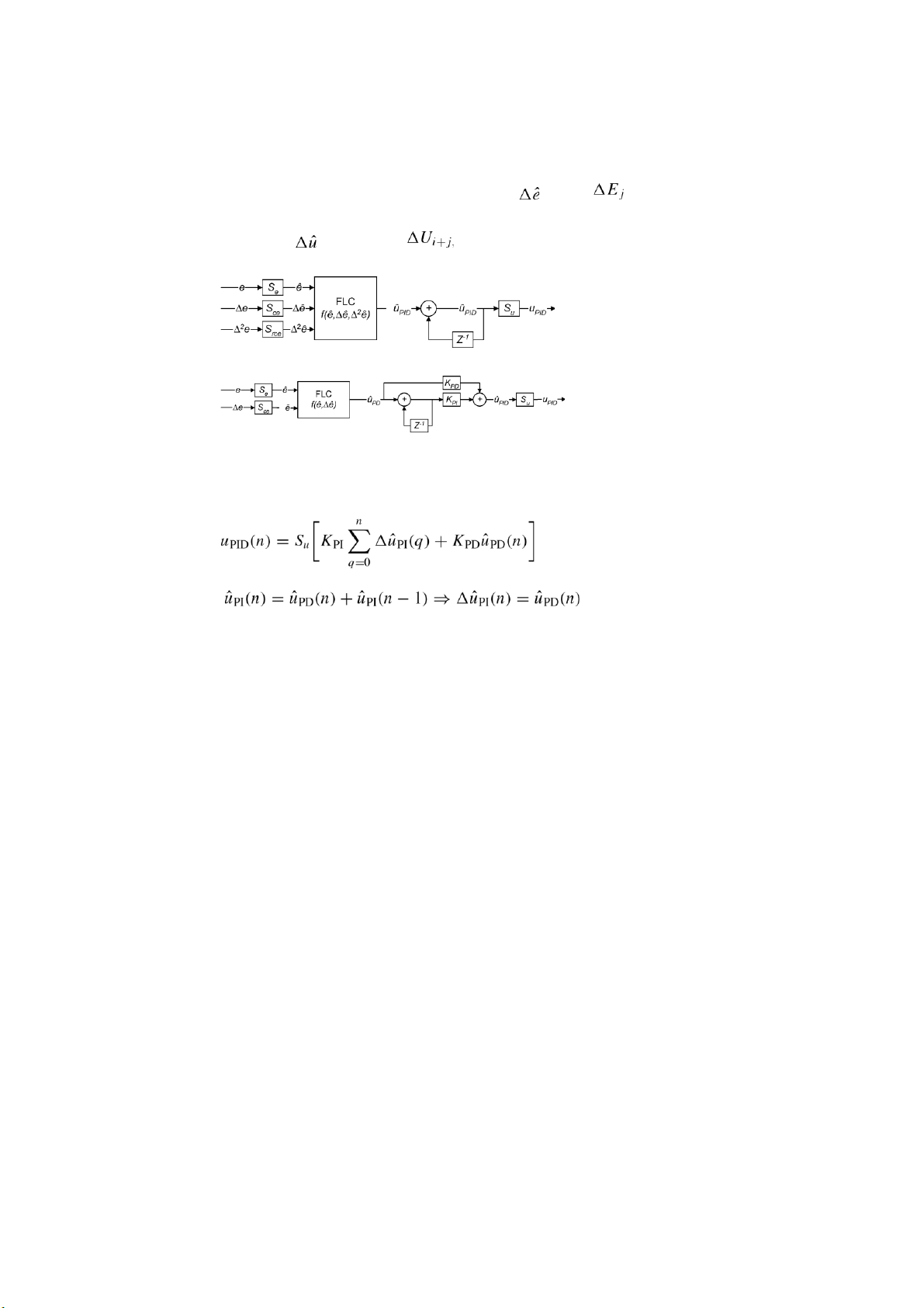
3.1. THREE-INPUT FUZZY LOGIC CONTROLLER (FLC) STRUCTURE WITH COUPLED RULE The inputs are ê(n), , and
, corresponding to an incremental type
fuzzy PID controller as shown in Figure 3.
The rule base structure can be expressed by: IF eˆ IS Ei AND IS AND IS . THENPID ISPID
The final PID control output is produced after taking the cumulative sum of the
FLC output given by expression (4). (q). (4)
3.2. TWO-INPUT FLC STRUCTURE WITH COUPLED RULE Having the inputs eˆ and
as the useful PID elements for fuzzy control, by
combining both PI and PD actions as shown in Figure 4, a two-input fuzzy PID
controller can be formed. The rule base structure is identical to Mamdani-type fuzzy PI controller. lOMoAR cPSD| 58675420 304 G. M. KHOURY ET AL.
The basic rule base of this conventional type is given by: ELSEIF eˆ IS Ei AND IS . i,j THEN PD IS PD
Figure 3. Three-input fuzzy PID controller.
Figure 4. Two-input fuzzy PID controller.
With the additional gains KPD and KPI, the final PID control signal shown in Figure 4 is given by expression (5). , (5) where . 3.3. INFERENCE SYSTEM
The output of each fuzzy inference system is derived using the standard Zadeh–
Mamdani’s min–max gravity reasoning method.
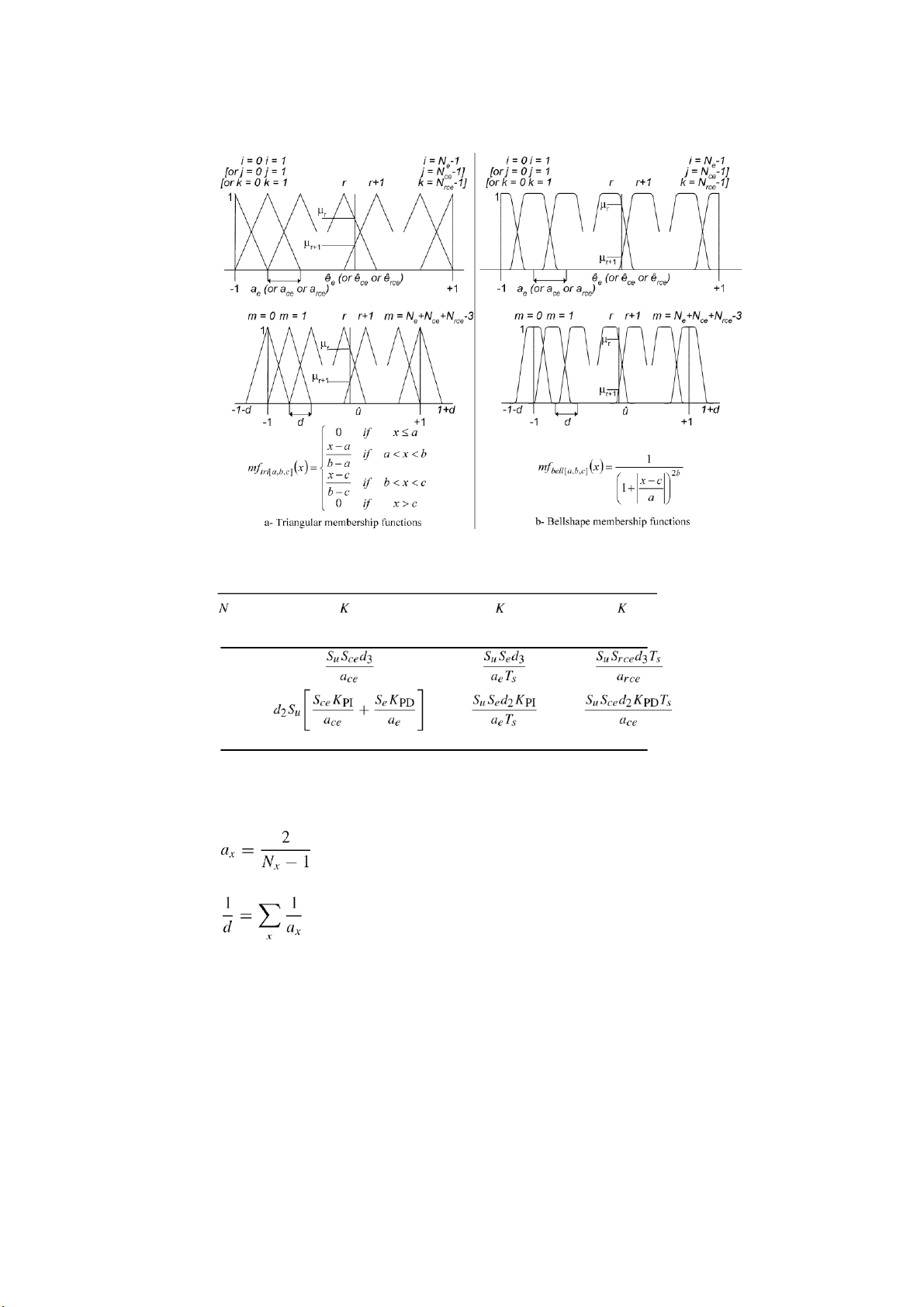
The universe of discourse of each input variable is defined to be within the
range [−1,1]. For simplicity we will use symetrical triangulare or bellshape
membership functions as shown in Figure 5. Any other symetrical shape
membership function can be used. Let ax be the corresponding distances between
two adjacent input memebership functions for the fuzzy input x. The output
linguistic variables are defined within the universe of discourse of [(−1 − d),(1 +
d)] where d is the distance between two adjacent output membership functions. The factor d is derived lOMoAR cPSD| 58675420
FUZZY PID CONTROL OF A FIVE DOF ROBOT ARM 305
Figure 5. Membership functions’ distribution of fuzzy inputs and output of a three inputs fuzzy PID.
Table I. Apparent linear gains for the three and two-input fuzzy PID controllers Pa Ia Da 3 2
from the choice of the number of membership functions Nx of the input variables x via the formulas: , (6) . (7) lOMoAR cPSD| 58675420 306 G. M. KHOURY ET AL. 3.4. TUNING LEVELS
Any fuzzy PID structure together with its fuzzy knowledge base usually results in nonlinear PID actions.
The first level of tuning relates to the normalized nonlinear characteristics and
is usually obtained by changing the knowledge base parameters of the fuzzy system.
The second level of tuning is related to scale factors and other gain parameters
used in constructing the fuzzy PID system. This second tuning level determines
the overall characteristics of the controller. For this purpose, we define the so
called PID apparent linear gain (ALG) terms: KPa, KIa, and KDa. Note that the
definition of the ALG terms in [8] imposes that (1) the universes of discourse of
all input variables are uniformely partitionned; (2) the membership functions are
placed with 50% overlap supports and; (3) the rules are defined in a linear form.
In practice, the choice of the ALG terms is a trial and error tuning process.
However, the behavior of these gains is expected to be linearly equivalent to
conventional PID gains. A pole placement method [9] could therefore be used to
determine the values of the ALG terms. Once these values are obtained, the scale
factors and structural gains could be deduced. Other tuning methods are also
studied in [10, 16] and [17]. Table I, where N is the number of fuzzy inputs, gives
the ALG terms for the two PID structures used in this paper.
4. Integration of the Fuzzy PID Controller in the Control Loop
The dynamic model of the Maker 100 shows important nonlinearities. For each
joint an individual PID controller will be used. In this respect, it should be
emphasized that the coupling effects between the joints are not thus taken into
consideration by the controller. Clearly, this is a difficulty, which is to be alleviated
by the fuzzy PID controller by means of the nonlinearity of its inference system.
A similar uncoupled structure of fuzzy controllers is used in [4] for the tracking
problem of a two DOF robot arm. The study proved to be a success (maximum
peak to peak relative position error of 0.158%) of the tracking loop thanks to an
online mechanism of adjustment on the aggregation operator of rule premises.
The control will take place on the state variables in the joint space. Each joint
has it’s own PID controller. The control action of the fuzzy PID controllers was
scaled to a torque control action apllied to the Maker’s dynamique model, the
denormalization factor Su was so multiplied by a scaling factor of 10. For
simplicity, the parameters of those controllers are fixed similarly. This choice
eliminates the possibility of refining the control on some DOF more than on others.
Moreover, the choice of the same parameters for an angle measured in degrees and
a distance measured in meters is somehow unreasonable, but the fact that the lOMoAR cPSD| 58675420
FUZZY PID CONTROL OF A FIVE DOF ROBOT ARM 307
tracking position error should stay relatively small makes all DOF comparable.
However, this assumption will have to be verified later.
On the other hand, the attribution of numerical values for the normalization and
denormalization factors is largely related to the amount of error acceptable in the
feedback system. Enlarging the input interval [−1/Sx,1/Sx] to all the admissible
position error [−Emax-admissible,Emax-admissible], where Emax-admissible corresponds to the
maximal applicable step reference input to the joint state variable x, (i.e. Emax-
admissible = max[Xdesired-reference-position − Xactual-measured-position] over the whole working
space of the corresponding joint), will increase the tracking performance for the
maximal step reference input but will largely decrease its sensitivity and
performance towards small displacements of this joint. In fact, if the normalization
was tuned to increase the control sensitivity towards large displacements of the
corresponding joint, a small displacement of this joint will only involve a limited
number of membership functions, those located around zero, and consequently
only a few rules will be activated throughout the whole trajectory tracking
problem. Moreover, if the user seeks precision rather than speed, he should apply
a position step reference relatively close to the joint’s actual position. For this last
purpose, a fine trajectory generation should be used in order to optimize the overall
performance of the closed loop system.
In this paper, the tracking trajectory in the end-effector space is assumed to be
linear since the majority of robotic applications requier linear trajectories in their
working space. In fact, the robot follows the triangle reference trajectory defined
in the next section. The trajectory generation is based on the Bounded Deviation
Method [11], which was proposed by Taylor in [14], using third order polynomial
sub-trajectories [12] and a boundary of precision of 0.001 m on the Cartesian
endeffector trajectory around the theoretical desired linear trajectory.
5. Numerical Simulation of the Fuzzy Control System
The trajectory has a triangular form. The Cartesian coordinates of its corners are
listed in Table II where p stands for the pitch and r for the roll. The manipulator’s
end-effector will make a full turn of the trajectory in 20 s.
The trajectory generator, the five fuzzy PID controllers and the dynamic model
of the Maker 100 were simulated using Matlab/Simulink [15]. The sampling time
Ts is chosen to be 0.001 s for all simulations.
The performance of the fuzzy PID controllers were tested via two error
variables: (1) the absolute average position tracking error e¯i and (2) the relative
peakto-peak position tracking error eipp. The reader is invited to consult Appendix
B for the definition of these two error variables. lOMoAR cPSD| 58675420 308 G. M. KHOURY ET AL.
5.1. TWO-INPUT FUZZY PID CONTROLLER – KNOWLEDGE BASE DIMENSIONS
After a performance optimization sequence of trials, a preliminary study on the
effect of the number of rules in the inference system for the two input fuzzy PID
was held for multiple cases of rule base dimensions. Table III summarises the
different simulation results in the case of triangular membership functions.
Table II. Desired trajectory Point x (m) y (m) z (m) p (radian) r (radian) A 0.4 0.4 0.4 0 0 B 0.6 0 0 −π/2 π/20 C 0 0.6 0 −π/4 π
Table III. Position tracking errors for multiple cases of rule base dimensions Inference system
Relative peak-to-peak position tracking errors in parameters the joint space N1 N2 NRules e1pp (%) e2pp (%) e3pp (%) e4pp (%) e5pp (%) 3 3 9 0.0034 0.0030 0.0180 0.0039 0.0001 3 7 21 0.0024 0.0029 0.0108 0.0023 0.0078 5 5 25 0.0030 0.0025 0.0157 0.0034 0.0001 5 9 45 0.0022 0.0025 0.0110 0.0023 0.0156 7 3 21 0.0055 0.0046 0.0312 0.0069 0.0001 7 7 49 0.0026 0.0023 0.0142 0.0030 0.0005 9 5 45 0.0038 0.0027 0.0209 0.0046 0.0001 9 9 81 0.0026 0.0022 0.0148 0.0030 0.0005
It is clear from the tracking errors in Table III that, excluding the fifth degree
of freedom, the tracking precision is improved by increasing the number of
membership functions per fuzzy input. This is a direct result to the increase of
precision in the repartition of membership functions along the universe of
discourse of fuzzy inputs. On the other hand, enlarging the rule base dimension
will not only increase the nonlinearities of the fuzzy inference system but will also
slow down the response of the numerical controllers. In fact, for the inference
system to be easily acquired by the designer, it is more suitable to limit its
dimension since the tracking precision improvement is around 25% for an
enlargement of the rule base dimension of 800% (9 rules versus 81 rules fuzzy knowledge base). lOMoAR cPSD| 58675420
FUZZY PID CONTROL OF A FIVE DOF ROBOT ARM 309
By comparing cases of equal and non-equal numbers of membership functions
per fuzzy input, it is obvious that an increase in precision on the “change of error”
fuzzy input, {N1 = 3 and N2 = 7}, provides improvement on the tracking errors better
than that of enlarging precisions on both fuzzy inputs, {N1 = 7 and N2 = 7} and even
{N1 = 9 and N2 = 9}. This case is true for the first, third and fourth joint variables
where the improvement of the precision reaches 40% (on the fourth joint variable)
for an enlargement of the rule base dimension of 130% ({N1 = 3 and N2 = 7} versus
{N1 = 3 and N2 = 3}). However, this is not true for the second joint variable which
precision slightly improves and for the fifth joint variable which precision considerably decraeses.
As for the behavior of the fifth joint variable, unlike all othe joint variables, it
shows a non-dependancy towards the precision on the “error” fuzzy input and an
inversed dependancy towards its “change of error” membership functions ditribution precision.
The end-user is therefore invited to take advantage of the offered diversity on
the performances of the trajectory tracking problem on the five degrees of freedom
by tuning the fuzzy inference system parameters according to his application’s needs.
Finally, as a compromise and in order to emphasize the effect of the parameters
discussed below, unless otherwise mentionned, the case of {N1 = 3 and N2 = 3} will be used.
5.2. TWO-INPUT FUZZY PID CONTROLLER – MEMBERSHIP FUNCTIONS SHAPE
With the two inputs PID controller, a set of trial and error simulations led to the
optimization of the tracking problem. The values of the PID parameters are listed
in Table IV while the corresponding tracking error values for the five DOF are
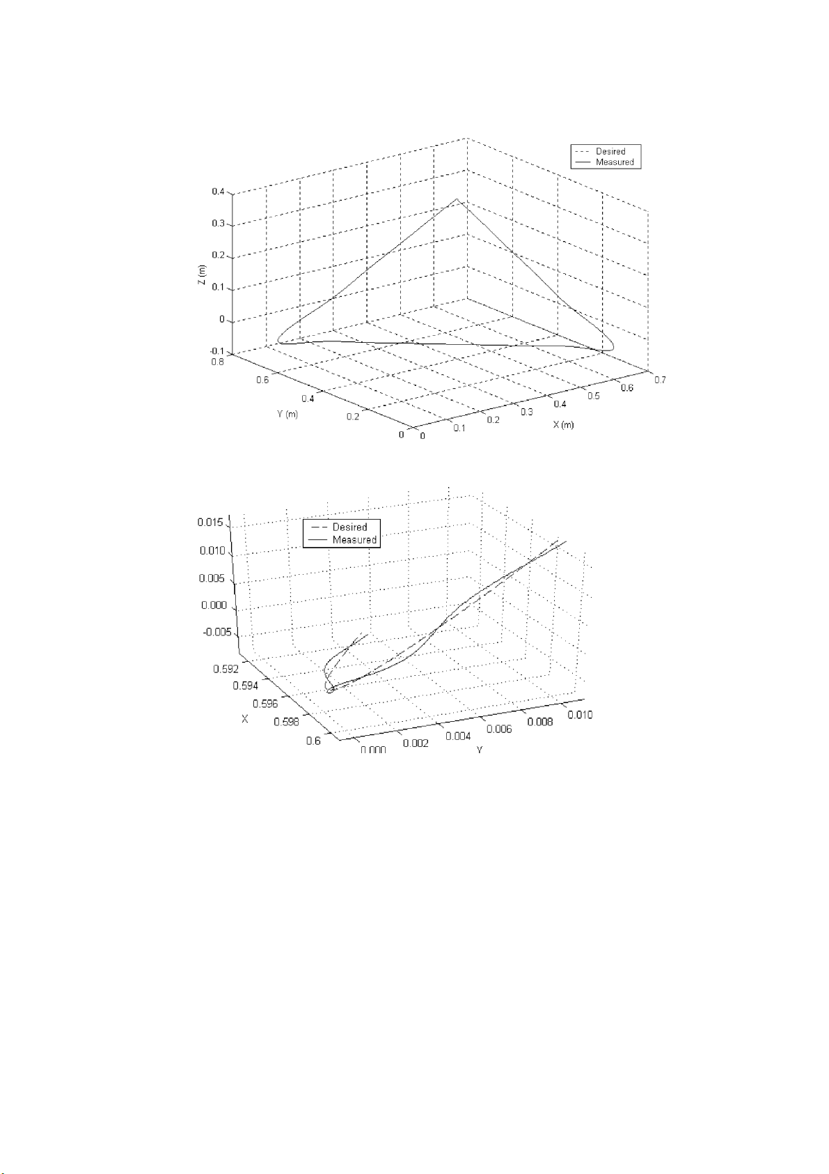
shown in Table V for multiple cases of membership function parameters. Figure 6
shows the desired and measured Cartesian trajectories of the manipulator’s
endeffector for the case of triangular membership functions with {N1 = 3; N2 = 3}
while Figure 7 gives a closer look to change in direction at point B (Table II) in
the case of bell shape membership functions with {N1 = 5; N2 = 5; b = 5}. The two
trajectories are superimposed in Figure 6 while the trajectory-tracking problem is
better illustrated in the case of Figure 7 where the performance is poorer. Figure 8
Table IV. Fuzzy PID controller tuning parameters Proportional integral gain KPI 7.97 Proportional derivate gain KPD 6.83 Denormalization factor Su 260 Normalization factor Se 5 lOMoAR cPSD| 58675420 310 G. M. KHOURY ET AL. Normalization factor Sce 2500
Table V. Position tracking errors for multiple cases of membership functions
Inference syst em pa ramete rs Absolute average
tion trackin g errors in th e joint posi space Membership N1 N2 b
e¯1 (deg) e¯2 (deg) e¯3 (mm) e¯4 (deg) e¯5 functions (deg) Triangular 3 3 – 0.0003 0.0002 0.0019 0.0001 0.0000 Triangular 5 5 – 0.0003 0.0002 0.0017 0.0001 0.0000 Bell shape 3 3 1 0.0008 0.0005 0.0045 0.0002 0.0000 Bell shape 3 3 5 0.0610 0.0613 0.1199 0.0229 0.0009 Bell shape 5 5 1 0.0007 0.0004 0.0038 0.0002 0.0000 Bell shape 5 5 5 0.0264 0.0265 0.0701 0.0098 0.0005 Inference system parameters
Relative peak-to-peak position tracking errors in the Cartesian space Membership N1 N2 b ex pp (%) ey pp (%) ezpp (%) eppp (%) er pp (%) functions Triangular 3 3 – 0.0035 0.0063 0.0085 0.0001 0.0026 Bell shape 3 3 1 0.0086 0.0149 0.0208 0.0002 0.0064
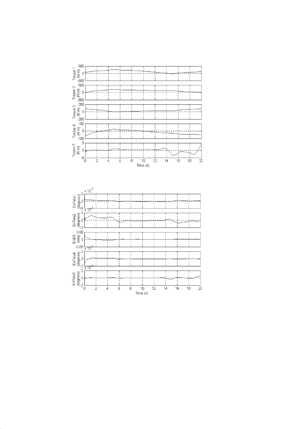
shows the instantaneous joint input torques and Figure 9 the resulting
instantaneous absolute position errors in the joint space for the case of triangular
membership functions with {N1 = 3; N2 = 3}.
Position tracking error values in Table V prove the success of the
implementation of the PID fuzzy control to the trajectory tracking problem of the
robotic arm. The use of triangular membership functions insures better
performences than that of bellshaped membership functions, the difference staying
negligeable and the range of position tracking errors being acceptable in both
cases. A closer look at the results obtained with the bell shape membership
functions shows that: (1) the more membership functions shapes are trapezoidal
{b = 5} the less performant the trajectory tracking problem will be; and vice versa,
(2) the more they are triangular {b = 1}, the closer the results are to those obtained with triangular membership lOMoAR cPSD| 58675420
FUZZY PID CONTROL OF A FIVE DOF ROBOT ARM 311
Figure 6. Desired and measured Cartesian trajectories of the end-effector. Case of triangular
membership functions with {N1 = 3; N2 = 3}.
Figure 7. Desired and measured Cartesian trajectories of the end-effector. Case of bell shape
membership functions with {N1 = 5; N2 = 5; b = 5}.
functions. This leads to conclude that the behavior of fuzzy PID controllers using
bellshape membership functions tends to that of fuzzy PID’s using triangular
membership functions. This last behavior makes the triangular membership lOMoAR cPSD| 58675420 312 G. M. KHOURY ET AL.
function seems like the best-matching solution for the trajectory tracking problem of the Maker 100.
Figure 8. Instantaneous joint input torques. Case of triangular membership functions with {N1 = 3; N2 = 3}.
Figure 9. Instantaneous absolute position errors in the joint space. Case of triangular
membership functions with {N1 = 3; N2 = 3}. lOMoAR cPSD| 58675420
FUZZY PID CONTROL OF A FIVE DOF ROBOT ARM 313
Although the tracking problem seems close to perfection, the rate of acceptable
error on the manipulator’s end-effector position is a function of the precision
required by the task at hand and is limited by the mechanical and electrical
performances of the joints’ actuators.
5.3. TWO-INPUT FUZZY PID CONTROLLER – ROBUSTNESS STUDY
5.3.1. Towards Change of Trajectory
Keeping the same tuning for the fuzzy PID controllers as adjusted for the triangular
trajectory tracking with triangular membership functions and three membership
functions per fuzzy input, the robot arm was tested for a different form of linear trajectory (Table VI).
Measured tracking errors listed in Table VII illustrate the ability of the tuned
fuzzy PID controllers to ensure the success of the trajectory tracking problem of
the Maker 100 within its working space. Other trajectory trackings could also be
verified using the same tuning of the fuzzy PID controllers.
5.3.2. Towards Change of Robot Parameters
In these simulations, the control loop was tested in presence of uncertanities in the
robot arm’s model. In each simulation, using triangular trajectory of Table II and
the previously tuned PID controllers, one or more of the Maker’s nineteen
parameters was made subject to variations throughout the trajectory tracking
problem. Results of the different cases are listed in Table VIII where uncertainities
were added to frictions F1, F4 and F5, mass m5 and centre of mass z5.
The simulation results show the robustness of the proposed fuzzy PID control
towards uncertanities affecting the Robot mechanical parameters.
It should be mentionned that all the previous developments can be extended
easily to the three inputs fuzzy PID controllers case.
Table VI. Desired trajectory Point x (m) y (m) z (m) p (radian) r (radian) A 0.3 0.6 0.4 0 π B 0.5 0.5 0.1 −π π/2 C 0 0.6 0 −π/4 π D 0.3 0.4 0.2 π/4 0 E 0.3 0.1 0.8 −π/3 π/4
Table VII. Position tracking errors for multiple trajectories lOMoAR cPSD| 58675420 314 G. M. KHOURY ET AL. Trajectory
Relative peak-to-peak position tracking errors in the Cartesian space ex pp (%) ey pp (%) ezpp (%) eppp (%) er pp (%) Table II 0.0035 0.0063 0.0085 0.0001 0.0026 Table VI 0.0047 0.0103 0.0045 0.0001 0.0031
Table VIII. Position tracking errors for multiple cases of uncertainities within the robot dynamic model Perturbation
Relative average position tracking errors in the joint space
e1pp (%) e2pp (%) e3pp (%) e4pp (%) e5pp (%) None
0.0034 0.0030 0.0180 0.0039 0.0001
F1 starts increasing at t = 4 s with a slope
of 10 and stops at t = 13.37 s
0.0036 0.0030 0.0180 0.0039 0.0001
F4 starts increasing at t = 5 s with a slope of 8 and stops at t = 13.25 s
F5 starts increasing at t = 6 s with a slope
of 10 and stops at t = 15.78 s
0.0034 0.0030 0.0180 0.0039 0.0009
m5 steps at t = 6 s to 5 times m5 z5
steps at t = 6 s to 5 times z5
0.0038 0.0567 0.0180 0.0311 0.0001
5.4. THREE-INPUT FUZZY PID CONTROLLER – TUNING METHOD
In the case of the three inputs fuzzy PID structure, the choice of the PID parameters
was made possible by a pole placement method [9]. First, we consider the dynamic
behavior of the position tracking error to be similar to its behavor in a Computed
Torque Control, and which is given by: . (8)
By substituting Equation (8) by its Laplace equivalent, we obtain: (s3 + K (9) Ds2 + KP s + KI)E(s)ˆ = 0.
Equation (9) could be rewritten [6] as Equation (10): lOMoAR cPSD| 58675420
FUZZY PID CONTROL OF A FIVE DOF ROBOT ARM 315 , (10)
where: α is a positive real number for the dynamic behavior of the position error
to be stable, ξ is the damping ratio, wn is the natural pulsation, ts is the settling time
defined as the time by witch the second order system response enters for the last
time from the top or the buttom the band [95%;105%] of the step refernce input.
The dynamic behavior of the position error is thus governed by the choice of
its three poles which will lead us to the desired proportional, integral and derivate
gains. By identifying these gains to the ALG terms of the three inputs fuzzy PID
Table IX. Fuzzy PID controller tuning procedure
Pole placement for the dynamic behavior of the position error Alpha (real pole) α 5ξwn Response time (s) tr 0.3 Damping ratio ξ 0.5
Computation of the equivalent linear PID gains Apparent proportional gain KPa 1533.3 Apparent integral gain KIa 22923 Apparent derivate gain KDa 73.2567
Choice of the first normalization factor Normalization factor Se 1/0.2
Deduction of the other scale factors Denormalization factor Su 13.7540 Normalization factor Sce 334.4404 Normalization factor Srce 15979 lOMoAR cPSD| 58675420 316 G. M. KHOURY ET AL.
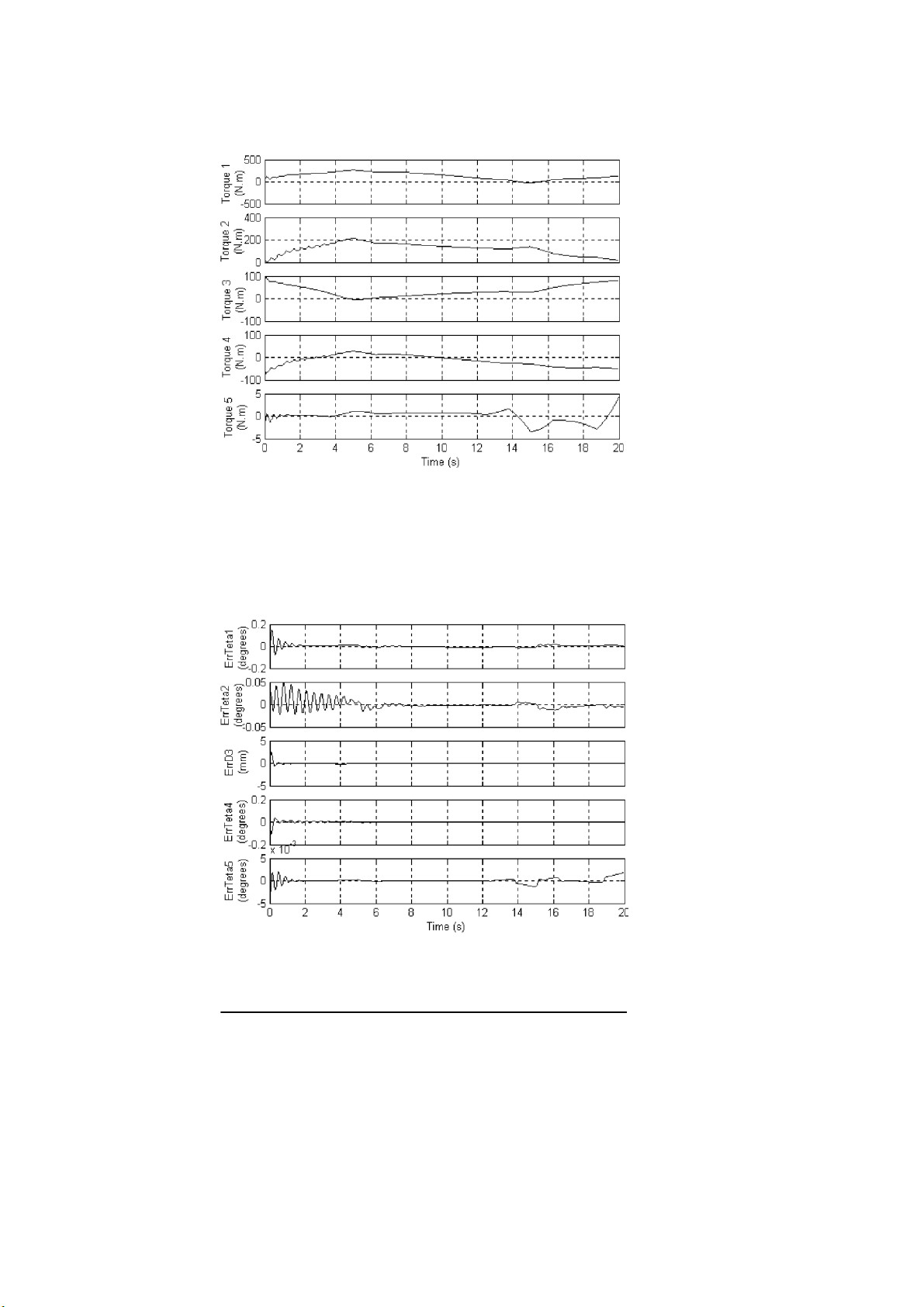
Figure 10. Instantaneous joint input torques.
structure, the values of the normalization and denormalization factors will be
obtained obtained. Table IX summarizes this tuning procedure.
Figure 10 shows the instantaneous joint input torques and Figure 11 the
resulting instantaneous position absolute errors in the joint space for the case of
Figure 11. Instantaneous absolute position errors in the joint space.
Table X. Position tracking errors lOMoAR cPSD| 58675420
FUZZY PID CONTROL OF A FIVE DOF ROBOT ARM 317
Absolute average position tracking errors in the joint space e¯1 (deg) e¯2 (deg) e¯3 (mm) e¯4 (deg) e¯5 (deg) 0.0089 0.0063 0.0539 0.0031 0.0003
Relative peak-to-peak position tracking errors in the joint space e1pp (%) e2pp (%) e3pp (%) e4pp (%) e5pp (%) 0.2452 0.1919 1.1833 0.2550 0.0026
triangular membership functions with {N1 = 3; N2 = 3; N3 = 3} Table X gives the
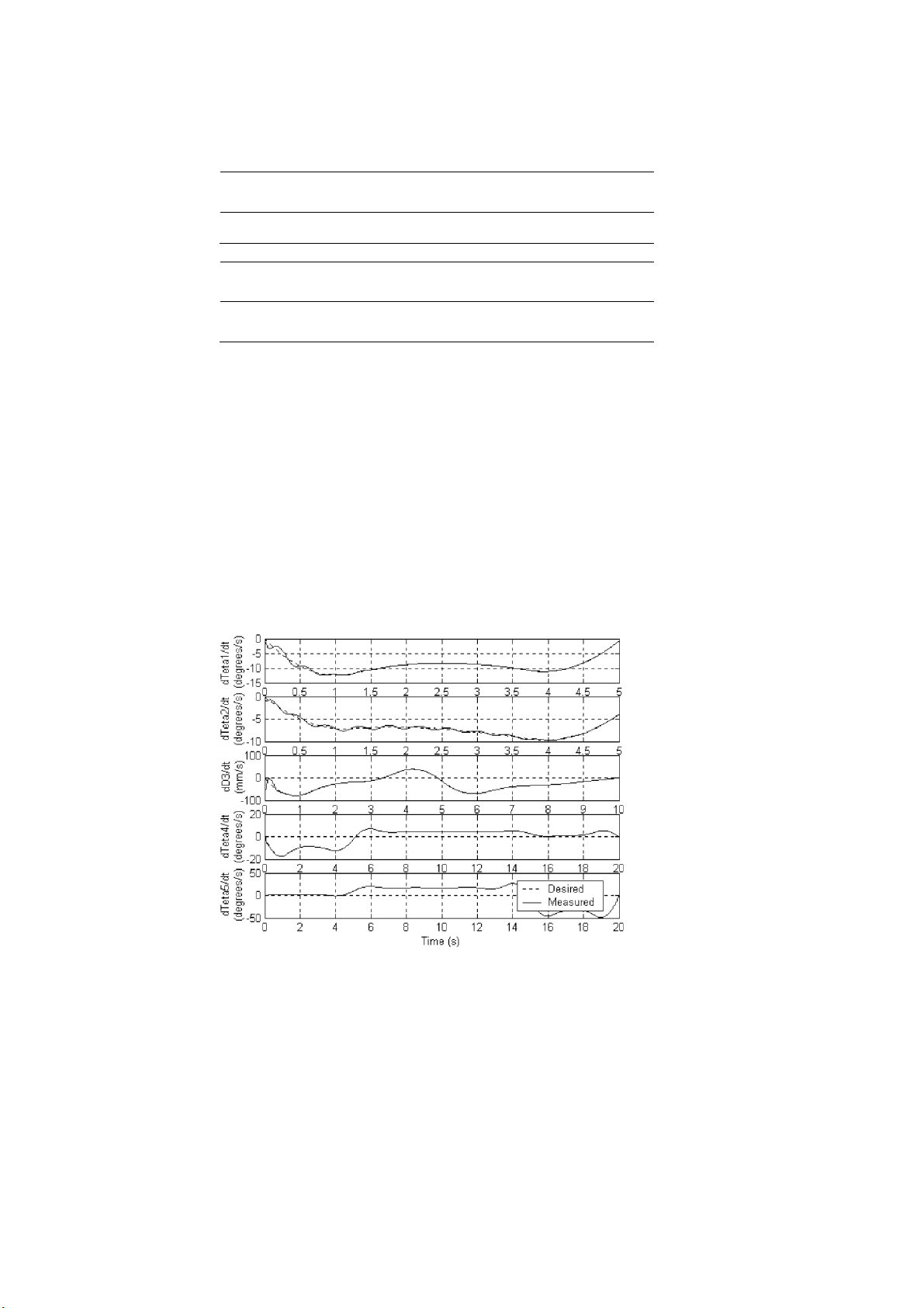
resulting tracking error variables. Figure 12 shows the desired and measured
variations of the velocities in the joint space. The velocity variations illustrate the
tracking dynamics of the control loop. They show a transient oscillatory behavior
around the desired velocity reference. This transient phase is then followed by the
convergence of the velocity to its desired instantaneous value.
6. Comparison to Other Nonlinear Controls
Using the same simulated dynamic model of the Maker 100, the computed torque
and the direct adaptive control methods [12, 13] were simulated. For a more
realistic simulation, the Maker’s parameters used in the computed torque control
were taken equal to 1.1 times those of the simulated dynamic model of the Maker 100.
Figure 12. Instantaneous joint velocities in the joint space.
Table XI. Position tracking errors lOMoAR cPSD| 58675420 318 G. M. KHOURY ET AL. Control method
Absolute average position tracking errors in the joint space e¯1 (deg) e¯2 (deg) e¯3 (mm) e¯4 (deg) e¯5 (deg) Computed torque 1.3e−5 1.5e−5 1.5e−3 6e−5 2.5e−5 Direct adaptive 0.1e−3 0.1e−3 6.7e−3 0.2e−3 0.1e−3 Fuzzy 2-input PID 0.3e−3 0.2e−3 1.9e−3 0.1e−3 0.0e−3 Fuzzy 3-input PID 8.9e−3 6.3e−3 53.9e−3 3.1e−3 0.3e−3
Similarly, the initial values for the parameters’ estimation algorithm in the adaptive
control were taken 1.5 times those of the simulated dynamic model. The sampling
time Ts was chosen to be 0.001 s for all simulations. The performances of the fuzzy
PID controls are evaluated by examining the error variables listed in Table XI.
The errors obtained with the two fuzzy PID controllers are acceptable. Even
though the two-input structure provides better performance in term of tracking
errors, the three-input structure offers the advantage of a simpler and clearer tuning
procedure and so seems more interesting to use.
The performances provided by the computed torque and the direct adaptive
controls overpass those of the fuzzy PID controllers. However these performances
are limited to the simulation case where the adoption of a simulated dynamic
model similar for both the controller design and the controlled model offers
optimized working conditions for the tracking problem. And on the other hand, in
the real case, the manipulator’s dynamic parameters are partially unknown and
could not be known with high precision.
The tracking simulated errors are therefore the most realistic in the case of the
fuzzy PID controllers. This criteria represents the main advantage of the fuzzy
control approach, i.e. its non-dependency on the dynamic model of the plant. 7. Conclusion
This paper studied the design and performances of the DA fuzzy PID control
method on a five DOF robot arm. The study confirmed the success of the proposed
fuzzy control laws. The major difference between the two used fuzzy PID
structures was revealed in their tuning procedures. With the three-input structure,
the pole placement method along with the use of the structure’s apparent linear
gains allowed numerical calculation of it’s tuning parameters, avoiding so the trial
and error procedures usually used in fuzzy control design methods. A comparative
study of the designed fuzzy control to other nonlinear controls confirmed again
the success of the fuzzy tracking control system.