Graph Theory chuyên đề Toán | Trường Đại học Sư phạm Hà Nội
Graph Theory chuyên đề Toán | Trường Đại học Sư phạm Hà Nộivới những kiến thức và thông tin bổ ích giúp sinh viên tham khảo, ôn luyện và phục vụ nhu cầu học tập của mình cụ thể là có định hướng, ôn tập, nắm vững kiến thức môn học và làm bài tốt trong những bài kiểm tra, bài tiểu luận, bài tập kết thúc học phần, từ đó học tập tốt và có kết quả cao cũng như có thể vận dụng tốt những kiến thức mình đã học vào thực tiễn cuộc sống.
Môn: Chuyên đề Toán 64 tài liệu
Trường: Trường Đại học Sư Phạm Hà Nội 3.3 K tài liệu
Tác giả:


Preview text:
Introduction
Lecture 1 – Graph Theory 2016 – EPFL – Frank de Zeeuw 1 Definitions
Definition. A graph G = (V, E) consists of a finite set V and a set E of two-element subsets
of V . The elements of V are called vertices and the elements of E are called edges.
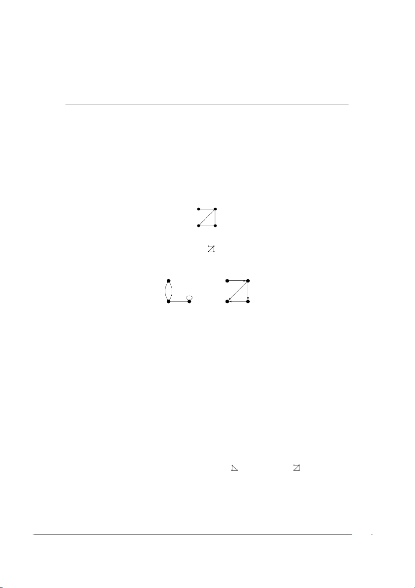
For instance, very formally we can introduce a graph like this: V = {1, 2, 3, 4},
E = {{1, 2}, {3, 4}, {2, 3}, {2, 4}}.
In practice we more often think of a drawing like this: 1 2 4 3
Technically, this is what is called a labelled graph, but we often omit the labels. When we
say something about an unlabelled graph like
, we mean that the statement holds for any labelling of the vertices.
Here are two examples of related objects that in this course we do not consider graphs:
The first is a multigraph, which can have multiple edges and loops; the corresponding def-
inition would allow the edge set and the edges to be multisets. The second is a directed
graph, in which every edge has a direction; in the corresponding definition the edges would
be ordered pairs instead of two-element subsets. In this course we mostly avoid these variants
for simplicity, although they are certainly very useful objects. Most facts about graphs in
our sense have analogues for multigraphs or directed graphs, although those are often a bit
less nice. Another type of graph that we are avoiding is infinite graphs; many facts about
finite graphs do not extend to infinite graphs.
Some notation: Given a graph G, we write V (G) for the vertex set, and E(G) for the
edge set. For an edge {x, y} ∈ E(G), we usually write xy, and we consider yx to be the same
edge. If xy ∈ E(G), then we say that x, y ∈ V (G) are adjacent or connected or that they are
neighbors. If x ∈ e, then we say that x ∈ V (G) and e ∈ E(G) are incident.
Definition (Subgraphs). Two graphs G, G′ are isomorphic if there is a bijection ϕ : V (G) →
V (G′) such that xy ∈ E(G) if and only if ϕ(x)ϕ(y) ∈ E(G′). A graph H is a subgraph of a
graph G, denoted H ⊂ G, if there is a graph H′ isomorphic to H such that V (H′) ⊂ V (G) and E(H′) ⊂ E(H).
With this definition we can for instance say that is a subgraph of . As mentioned
above, when we talk about graphs we often omit the labels of the vertices. A more formal way
of doing this is to define an unlabelled graph to be an isomorphism class of labelled graphs.
We will be somewhat informal about this distinction, since it rarely leads to confusion. 1
Definition (Degree). Fix a graph G = (V, E). For v ∈ V , we write N (v) = {w ∈ V : vw ∈ E}
for the set of neighbors of v (which does not include v). Then d(v) = |N (v)| is the degree
of v. We write δ(G) for the minimum degree of a vertex in G, and ∆(G) for the maximum degree.
Definition (Examples). The following are some of the most common types of graphs.
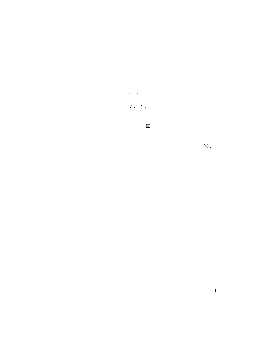
• Paths are the graphs Pn of the form
. The graph Pn has n edges and n + 1
vertices; we call n the length of the path.
• Cycles are the graphs Cn of the form
. The graph Cn has n edges and n
vertices; we call n the length of the cycle.
• The complete graphs are the graphs Kn on n vertices in which all vertices are adjacent. The graph K n has n edges. For instance, K 2 4 is .
• The complete bipartite graphs are the graphs Ks,t with a partition V (Ks,t) = X ∪ Y
with |X| = s, |Y | = t, such that every vertex of X is adjacent to every vertex of Y , and
there are no edges inside X or Y . Then Kst has st edges. For example, K2,3 is .
The following are the most common properties of graphs that we will consider.
Definition (Regular). A graph G is k-regular if d(v) = k for all v ∈ V (G).
Definition (Bipartite). A graph G is bipartite if there is a partition V (G) = X ∪ Y such
that every edge of G has one vertex in X and one in Y ; we call such a partition a bipartition.
Definition (Connected). A graph G is connected if for all x, y ∈ V (G) there is a path in G
from x to y (more formally, there is a path Pk which is a subgraph of G and whose endpoints are x and y).
A connected component of G is a maximal connected subgraph of G (i.e., a connected subgraph
that is not contained in any larger connected subgraph). The connected components of G form a partition of V (G). 2 Basic facts
In this section we prove some basic facts about graphs. It is a somewhat arbitrary collection
of statements, but we introduce them here to get used to the terminology and to see some typical proof techniques. X
Proposition 2.1. In any graph G we have d(v) = 2|E(G)|. v∈V (G)
Proof. We double count the number of pairs (v, e) ∈ V (G) × E(G) such that v ∈ e. On
the one hand, a vertex v is involved in d(v) such pairs, so the total number of such pairs is P
d(v). On the other hand, every edge is involved in two such pairs, so the number of v∈V (G) pairs must equal 2|E(G)|. 2
This fact is sometimes called the “handshake lemma” because it says that at a party the
number of shaken hands is twice the number of handshakes. It has useful corollaries, such as
the fact that the number of odd-degree vertices in a graph must be even.
The next lemma gives a condition under which a graph must contain a long path or cycle.
Note that “contains a path” means that the graph has a subgraph that is isomorphic to some
Pn, and similarly for cycles. The proof is an example of an extremal argument, where we take
an object that is extremal with respect to some property, and show that this extremality
implies some other property of the object.
Proposition 2.2. A graph G with minimum degree δ(G) ≥ 2 contains a path of length at
least δ(G) and a cycle of length at least δ(G) + 1.
Proof. Let v1 · · · vk be a maximal path in G, i.e., a path that cannot be extended. Then any
neighbor of v1 must be on the path, since otherwise we could extend it. Since v1 has at least
δ(G) neighbors, the set {v2, . . . , vk} must contain at least δ(G) elements. Hence k ≥ δ(G)+1,
so the path has length at least δ(G).
To find a long cycle, we continue the proof above. The neighbor of v1 that is furthest
along the path must be vi with i ≥ δ(G) + 1. Then v1 · · · viv1 is a cycle of length at least δ(G) + 1.
Note that in general these bounds cannot be improved, because Kδ+1 has minimum degree
δ, but its longest path has length δ and its longest cycle has length δ + 1. In Problem Set 1
we will see that we can find longer paths in graphs that are not complete.
The following lemma can be helpful when trying to prove certain statements for general
graphs that are easier to prove for bipartite graphs. The lemma says that you don’t have to
remove more than half the edges of a graph to make it bipartite. The proof is an example of
an algorithmic proof, where we prove the existence of an object by giving an algorithm that constructs such an object.
Proposition 2.3. Any graph G contains a bipartite subgraph H with |E(H)| ≥ |E(G)|/2.
Proof. We prove the stronger claim that G has a bipartite subgraph H with V (H) = V (G)
and dH(v) ≥ dG(v)/2 for all v ∈ V (G). Starting with an arbitrary partition V (G) = X ∪ Y
(which need not be a bipartition for G), we apply the following procedure. We refer to X
and Y as “parts”. For any v ∈ V (G), we see if it has more edges to X or to Y ; if it has more
edges that connect it to the part it is in than it has edges to the other part, then we move it
to the other part. We repeat this until there are no more vertices v that should be moved.
There are at most |V (G)| consecutive steps in which no vertex is moved, since if none of
the vertices can be moved, then we are done. When we move a vertex from one part to the
other, we increase the number of edges between X and Y (note that a vertex may move back
and forth between X and Y , but still the total number of edges between X and Y increases
in every step). It follows that this procedure terminates, since there are only finitely many
edges in the graph. When it has terminated, every vertex in X has at least half its edges
going to Y , and similarly every vertex in Y has at least half its edges going to X. Thus the
graph H with V (H) = V (G) and E(H) = {xy ∈ E(G) : x ∈ X, y ∈ Y } has the claimed
property that dH(v) ≥ dG(v)/2 for all v ∈ V (G). 3
The last lemma gives a characterization of bipartite graphs. An “odd cycle” is just a
cycle whose length is odd. Again we give an algorithmic proof.
Proposition 2.4. A graph is bipartite if and only if it contains no odd cycle.
Proof. Suppose that G is bipartite with bipartition V (G) = X ∪ Y , and that v1 · · · vkv1 is a
cycle in G, with v1 ∈ X. We must have vi ∈ X for all odd i and vi ∈ Y for all even i. Since
vk is adjacent to v1, it must be in Y , so k must be even and the cycle is not odd.
Suppose we have a connected graph G which has no odd cycles. We can obtain a bipar-
tition using the following algorithm. Start with X, Y being empty sets. Pick an arbitrary
vertex x0 and put it in X. Put all the neighbors of x0 in Y . For each y ∈ Y , put into X
all neighbors of y that have not yet been assigned. Then for each x ∈ X, put into Y all
neighbors that have not yet been assigned. Keep repeating this until all vertices have been
assigned. This algorithm is well-defined because no vertex is assigned more than once (thanks
to the stipulation that we only consider unassigned vertices). It remains to be shown that
the algorithm terminates (i.e., it does not go on endlessly), and that the resulting partition
is really a bipartition of V (G).
The algorithm terminates because G is connected (by assumption). Indeed, this means
that every y ∈ Y has a path yv1 · · · vkx0 to x0, and in every step at least one more vertex
from this past must get assigned.
Next we show that V (G) = X ∪ Y is a bipartition. Suppose that two vertices x1, x2 ∈ X
are adjacent. By construction, there is a path P from x1 to x0 that uses only edges between
X and Y , and similarly there is such a path P ′ from x2 to x0; note that these paths may
intersect, so their union might not be a path. Let x3 be the first vertex where P intersects
P ′ (this could be x0). Then we get a path P ′′ from x1 to x3 to x2 that also has the property
that all its edges are between X and Y . Since this path goes from X to X using only edges
between X and Y , it must have an even number of edges. Thus, if we combine it with x1x2,
we get an odd cycle, which is a contradiction. Similarly, if y1, y2 ∈ Y are adjacent, combining
this edge with the path from y1 to y2 gives an odd cycle. This shows that all edges of G are
between X and Y , so G is bipartite.
We did the above under the assumption that G is connected. If it is not, we can apply
the above to each connected component, and arbitrarily combine the bipartitions of the
components to get a bipartition of G. 4 ProblemSet1
GraphTheory2016–EPFL–FrankdeZeeuw&ClaudiuValculescu
Youcanhandinoneofthestar problemsbefore10:15amonThursdayMarch3rd.
1. Forsomen,giveagraphwithn vertices,n + 3edges,andexactly8cycles.
2. Findtwonon-isomorphicgraphswiththesamenumberofverticesandthesamesequence ofdegrees.
3. Showthatanygraphwithatleasttwoverticeshastwoverticeswiththesamedegree.
4. Whatisthemaximumnumberofedgesinabipartitegraph onn vertices? Proveit.
5. LetG beagraphinwhicheveryvertexhasevendegree. ShowthatE(G)canbeparti- tionedintotheedgesetsofcycles.
6. A graph is k-regular if every vertex has degree k. Describe all 1-regular graphs and all
2-regulargraphs. Showthatagraphonanoddnumberofverticescannotbe3-regular,
whileforeveryevenn ≥ 4,thereisa3-regulargraphonn vertices.
7. Showthatanygraphwithatleast6verticescontains3verticesthatarepairwiseadjacent,
or3verticesthatarepairwisenon-adjacent.
8. LetG beagraphcontainingacycleC,andassumethatG containsapathoflengthat √
leastk betweentwoverticesofC. ShowthatG containsacycleoflengthatleast k. √ √
*9. ProvethestatementofProblem8with 2k insteadof k.
*10. ShowthateveryconnectedgraphG containsapathoflengthatleastmin{2δ(G), |G|−1}. Trees
Lecture 2 – Graph Theory 2016 – EPFL – Frank de Zeeuw 1 Basic facts
Definition. A tree is a connected graph without cycles. A forest is a graph without cycles. In
a tree or a forest, a vertex of degree one is called a leaf.
Proposition 1.1. Every tree with at least two vertices has a leaf.
Proof. Take a longest path x0x1 · · · xk in the tree (so k ≥ 1, since the tree has at least two
vertices). A neighbor of x0 cannot be outside the path, since then the path could be extended.
But if x0 were adjacent to xi for some i>1, then x0x1 · · · xix0 would be a cycle. So the only
neighbor of x0 is x1, and x0 is a leaf. (Of course, the same works for xk, so there are at least two leaves.)
Proposition 1.2. Any tree T satisfies |E(T )| = |V (T )| − 1.
Proof. We use induction on the number of vertices. If |V (T )| = 1, then |E(T )| = 0. Otherwise,
Proposition 1.1 gives a leaf x0 of T . Let T ′ be the graph obtained by removing x0 and its only
edge. Then T ′ is connected, since for any x,y ∈ V (T ′) there is a path from x to y in T , and this
path cannot pass through x0, so it is also a path in T ′. Since T has no cycles, neither does T ′,
so T ′ is a tree. By induction we have |E(T ′)| = |V (T ′)| − 1, so plugging in |E(T ′)| = |E(T )| − 1
and |V (T ′)| = |V (T )| − 1 give the desired formula.
Corollary 1.3. Any forest F satisfies |E(F )| = |V (F )| − c(F ), where c(F ) is the number of connected components of F .
Proof. Each connected component T of F is a tree, so Proposition 1.2 gives |E(T )| = |V (T )|−1.
Summing up over the c(F ) components gives the desired formula.
Proposition 1.4. A graph G is a tree if and only if for all x,y ∈ V (G) there is a unique path between x and y.
Proof. First suppose we have a graph G in which any two vertices are connected by a unique
path. Then G is certainly connected. Moreover, if G contained a cycle x0x1 · · · xkx0, then x0xk
and x0x1 · · · xk would be two distinct paths between x0 and xk. Hence G is a tree.
Suppose G is a tree and x,y ∈ V (G). Since G is connected, there is at least one path from
x to y. Suppose there are two paths P 6= P ′ from x to y. If these paths only intersect at x and
y, we can immediately combine them into a cycle, but in general the paths could intersect in a
complicated way, so we have to be careful. The paths P and P ′ could start out from x being
the same; let u be the last vertex at which they are the same. Let v be the first vertex after u
on P that is again on P ′. Then there is a cycle that goes along P from u to v, and then back
along P ′ from v to u. This is a contradiction, so there is a unique path from x to y in G.
We introduce some notation for adding and removing edges in graphs. Given a graph G,
we write G + xyfor the graph with vertex set V (G) ∪ {x,y} and edge set E(G) ∪ {xy} (one or
both of x,y could already be in G). We also write G − xy for the graph with vertex set V (G) and edge set E(G)\{xy}. 1
Proposition 1.5. Let T be a tree. If xy∈ E(T ), then T − xy is not connected. If xy6∈ E(T )
and x,y ∈ V (T ), then T + xy contains a unique cycle.
Proof. Let xy∈ E(T ). Suppose that T − xyis connected. Then there is a path in T − xyfrom
x to y. Combining this path with xy gives a cycle contained in T , which is a contradiction.
Let xy6∈ E(T ) and x,y ∈ V (T ). By Proposition 1.4, there is a unique path in T from x to
y. Combining this path with xygives a cycle in T + xy. If there were a second cycle in T + xy,
it would also have to contain xy. Then removing xy from this cycle would give a second path
from x to y in T , contradicting the uniqueness of the path. 2
Spanning trees and basic algorithms
Definition. A spanning tree of a graph G is a tree T with |V (T )| = |V (G)|.
Proposition 2.1. A graph G is connected if and only if it has a spanning tree.
Proof. If G contains a spanning tree T , then any two vertices in V (G) are connected by a path
in T , which is also a path in G. Therefore G is connected.
If G is connected, the following algorithm shows that G has a spanning tree. Arbitrarily
pick x ∈ V (G) and consider it as a tree T . Repeat the following for as long as possible. For
every y ∈ V (G)\V (T ), check if y is adjacent to a vertex z in V (T ), and if so, replace T by T + yz.
The algorithm continues until V (T ) = V (G), at which point T is a spanning tree. Indeed,
it is a tree since every edge that we add has exactly one endpoint in the tree. It is spanning,
because if there is still a vertex y ∈ V (G)\V (T ) when the algorithm terminates, then the
connectedness of G implies that there is a path from y to x. Somewhere on this path there
must be a vertex v of T adjacent to a vertex w not in T , so the algorithm can still add w, and cannot have terminated.
The proof of Proposition 2.1 gives a very simple algorithm for finding a spanning tree. It is
of course not defined very formally; in particular, we did not specify how to pick y. We could
do that by putting an arbitrary order on V (G), and going over the vertices in that order.
Using this informal algorithm, we can give algorithms for the following basic tasks.
• Determine if G is connected: If the algorithm from the proof of Proposition 2.1 finds a
tree T with V (T ) = V (G), then G is connected; otherwise G is disconnected.
• Find the connected components of G: For a graph that is not connected, the algorithm will
find a spanning tree of a connected component of G; repeat this to get all the components.
• Determine if G contains a cycle: Find the connected components. If some connected
component H has |E(H)| 6= |V (H)| − 1, then it contains a cycle, because it contains a
spanning tree and at least one more edge. If |E(H)| = |V (H)| − 1 for every component,
then each component is equal to its own spanning tree, so the graph has no cycle. 3
Distances and breadth-first search
We saw one way of obtaining a spanning tree of a graph, but this is certainly not the only way.
We will now see a more specific algorithm that gives a spanning tree with special properties,
called a breadth-first search tree or BFS tree. This algorithm lets us answer various natural
questions, like determining the distance between two vertices. 2
Definition. Let G be a graph. For two vertices x,y ∈ V (G), the distance d(x,y) = dG(x,y) is
the length of a shortest path between x and y.
The diameter of G is the length of the longest shortest path: diam(G) = maxx,y∈V (G) d(x,y).
Given a graph G and a subgraph H ⊂ G, we define
∂(H) = {xy∈ E(G) : x ∈ V (H),y 6∈ V (H)}
for the set of edges going from vertices of H to vertices not in H. The algorithm in the proof of
Proposition 2.1 worked by repeatedly adding an edge from ∂(T ) to the current tree T . Another
bit of terminology: To single out one vertex of a tree, we refer to it as a root.
BFS Algorithm (given a graph G and a root r ∈ V (G))
(1) Let T be the graph consisting only of r; (2) Set S = ∂(T );
(3) For all xy∈ S, if T + xy does not contain a cycle, replace T by T + xy;
(4) If ∂(T ) 6= ∅, go back to (2);
(5) If |E(T )| = |V (G)| − 1, return T ; else return “disconnected”.
Proposition 3.1. Let G be a connected graph. The BFS Algorithm lets us find the shortest
path between any two vertices in G.
Proof. Let r,s ∈ V (G) be the vertices between which we want to find the shortest path. Run
the BFS Algorithm with root r. Give a vertex x the label f(x) = k if x was added to T
in the kth iteration of Step 3 (and label f(r) = 0). We prove by induction on f(x) that
f(x) = dT (r,x) = dG(r,x) for all x. It trivially holds for x = r.
If f(x) = k, then by construction x is adjacent (in T and G) to a vertex y with f(y) = k −1,
and by induction we have dT (r,y) = dG(r,y) = k − 1. So there is a path (in T and G) of length
k − 1 from r to y, which gives a path (in T and G) of length k from r to x. Moreover, there
cannot be a shorter path in G from r to x, because then dG(r,x) have f(x) = dG(r,x) Knowing that dT (r,x) = dG(r,x), we can find the shortest path from r to x in G by finding
the shortest path in T . To do that, we have to keep track of the “predecessor” of each x that
we add in step (3); i.e., the vertex p with f(p) = f(x) − 1 that x is connected to. Then, to
find the shortest path from r to s, we start from s and repeatedly take the predecessor, until we reach r.
Aside from letting us find shortest paths, the BFS algorithm lets us compute distances, and
it also gives us algorithms for the following tasks on G.
• Compute diam(G): For each pair of vertices, we can find a shortest path and thus the
distance. Do this for all pairs and take the largest distance.
• Find a shortest cycle in G: For every edge xy, find a shortest path between x and y in
G − xy (if it exists); combine this path with xy to get a cycle. Compare all these cycles to find the shortest. 3
Some of these algorithms are very inefficient, but they are already much better than brute
force approaches that go over all possible answers. There are all kinds of algorithms that do
these tasks faster, but in this course, we don’t care too much about efficiency, and we focus
on the graph-theoretical aspects (in particular, proving that the algorithms work). For more
sophisticated algorithms, we suggest taking a course in Combinatorial Optimization.
The problem of finding a shortest path is more interesting if we have a weight function P
w : E(G) → R+, and we want a path P for which the total weight w(e) is minimal. e∈P
The BFS algorithm above does not do this, because it finds a path with the fewest edges,
whereas a minimum-weight path may use many lightweight edges. Nevertheless, the best known
algorithm for finding minimum-weight paths, known as Dijkstra’s algorithm, is based on this BFS approach. 4 Minimum-weight spanning trees
Another natural algorithmic problem is the minimum-weight spanning tree problem. For a
graph G with a weight function w : E(G) → R+, we want a spanning tree T whose total P weight w(T ) =
w(e) is minimal (or determine that there is none, which means G is e∈E(T )
disconnected). It is easy to imagine an application with locations that have to be connected
by a network of roads, which has to be done with the total road length as small as possible.
The easiest thing to try is what is called a “greedy” approach: Repeatedly add the smallest
edge, while preserving connectedness and acyclicity (i.e., maintain a tree all along). Greedy Tree-Growing Algorithm
(1) Start with T being any vertex;
(2) Find e ∈ ∂(T ) with minimum w(e); if ∂(T ) = ∅, go to (4);
(3) Replace T by T + e; go to (2);
(4) If |E(T )| = |V (G)| − 1, return T , else return “disconnected”.
Theorem 4.1. The Tree-Growing Algorithm returns a minimum spanning tree, if it exists.
Proof. Suppose the algorithm returns T , and let e1,...,en−1 be the order in which the edges of
T are selected. Let T ∗ be a minimum-weight spanning tree that shares as many initial vertices
with T as possible; in other words, to each minimum-weight spanning tree T ∗ associate the
smallest i such that ei 6∈ T ∗, and choose the T ∗ with the largest i. If T = T ∗, then we are done, so assume T 6= T ∗.
Let e be the first edge not in T ∗ that was picked by the algorithm, and let T ′ be the tree
that the algorithm had before it picked e. Since e 6∈ T ∗, adding e to T ∗ creates a unique cycle
by Proposition 1.5. There must be an edge f 6= e in that cycle for which f ∈ ∂(T ′), since the
cycle leaves T ′ via e and must somehow re-enter T ′. Since the algorithm chose e over f, we must have w(e) ≤ w(f).
Now T ∗∗ = T ∗ + e − f is a tree (because the unique cycle containing e is broken by removing
f) with w(T ∗∗) ≤ w(T ∗), so T ∗∗ is also a minimum-weight spanning tree. But T ∗∗ shares more
initial vertices with T than T ∗, contradicting the definition of T ∗. It follows that T = T ∗, and T is minimum.
There are different greedy approaches for finding a minimum spanning tree, where a different
property is preserved in the process. In Problem Set 2, we will see two such algorithms, one that
greedily grows a forest, and one that greedily removes edges while keeping the graph connected. 4 ProblemSet2
Graph Theory 2016 – EPFL – Frank de Zeeuw & Claudiu Valculescu
Youcanhandinoneofthestar problemsbefore10:15amonThursdayMarch10th.
1. Prove that the following statements about a graph G are equivalent. - G is a tree;
- G is minimally connected (it is connected and removing any edge disconnects it);
- G is maximally acyclic (it has no cycles and adding any edge creates a cycle).
2. Show that every tree T has at least ∆(T ) leaves (vertices of degree 1).
3. Let T be a tree with |V (T )| ≥ 2. Suppose the vertices of T are colored red and blue,
such that no two adjacent vertices have the same color. Show that if there are at least as
many red vertices as blue vertices, then T has a red leaf.
4. Show that a graph G contains at least |E(G)| − |V (G)| + 1 cycles.
5. A vertex is central if its greatest distance from any other vertex is as small as possible.
Show that a tree has either a single central vertex, or two adjacent central vertices.
6. Determine the diameter of the following graphs.
- A hypercube, whose vertex set is {0, 1}d, with an edge between two vectors if they differ in exactly one entry;
- The Petersen graph, whose vertices are the 2-element subsets of {1, 2, 3, 4, 5}, with an
edge between two subsets if they are disjoint;
- A visibility graph, whose vertex set is a finite set X ⊂ R2, with an edge between two
points if they can see each other, i.e., if the line segment between them contains no other point of X.
7. Prove that the following Greedy Forest-Growing algorithm returns a minimum-weight
spanning tree, given a graph G and w : E(G) → R+.
Greedy Forest-Growing Algorithm
(1) Start with the empty graph F , and set S = E(G);
(2) Find e ∈ S with minimum w(e); if S = ∅ go to (4);
(3) Add e to F , unless that creates a cycle; remove e from S; go back to (2);
(4) If |E(F )| = |V (G)| − 1, return F , else return “disconnected”.
8. Design a “greedy removal” algorithm for minimum-weight spanning trees, which starts
with the whole graph and removes heavy edges. Prove that it works.
*9. Let T be a tree with t edges and G a graph. Prove that if |E(G)| ≥ t · |V (G)|, then T is a subgraph of G.
*10. Let X = {1,...,n} and let S be a set of n subsets of X. Use trees to prove that X
contains an element x such that adding it to the sets of S gives n distinct subsets. In
other words, there is an x ∈ X such that |{S ∪ {x} : S ∈ S}| = n. Covers and independent sets
Lecture 4 – Graph Theory 2016 – EPFL – Frank de Zeeuw 1
Summary of matchings in arbitrary graphs
In the previous lecture we treated matchings in bipartite graphs. As mentioned there, in this
course we will not cover matchings in arbitrary graphs, mostly because it would take too
much time. Nevertheless, we now give a quick overview of the basic facts about matchings in arbitrary graphs.
In an arbitrary graph, it is still true that a matching is maximum if and only if there is
no augmenting path for it (the proof that we gave did not use the bipartiteness). However,
the augmenting path algorithm that we described does not work, mainly because it is not
clear how to find an augmenting path or determine that none exists.
Both Hall’s Theorem and K¨onig’s Theorem fail for arbitrary graphs. Take for instance
the triangle K3. It is 2-regular, but does not have a perfect matching. The maximum size of
a matching is 1, but the minimum size of a vertex cover is 2.
There is an analogue of Hall’s Theorem for arbitary graphs, known as Tutte’s Theorem,
but it is more complicated. There is also a good algorithm due to Edmonds for finding a
maximum matching in an arbitrary graph, known as the “blossom algorithm”. It does use
augmenting paths, but its method for finding them is considerably more complicated. 2
Matchings, covers, and independent sets
In this section we discuss several objects in graphs related to matchings and covers.
Definition. LetG beagraph(thatisnotnecessarilybipartite).
-Amatching isasetM ⊂ E(G) suchthattheedgesinM arepairwisedisjoint;
-Avertex cover isasetC ⊂ V (G) suchthateveryedgeofG isincidenttoavertexofC;
-An independent set isasetI ⊂ V (G) suchthatnotwoverticesinI areadjacent;
- An edge cover is a set C ⊂ E(G) such that every vertex of G is incident to an edge in C
(notethatagraphwithanisolatedvertexhasnoedgecover).
Just like for matchings and vertex covers, we would like to find maximum independent
sets and minimum edge covers. We introduce the following parameters to keep track of all these extrema.
m(G) = max{|M| : M ⊂ E(G) is a matching}
vc(G) = min{|C| : C ⊂ V (G) is a vertex cover}
α(G) = max{|S| : S ⊂ V (G) is independent}
ec(G) = min{|C| : C ⊂ E(G) is an edge cover}
We now prove various relations between these parameters. 1
Tài liệu liên quan:
-

Đề cương ôn tập toán dành cho học sinh tiểu học
3 2 -
Bài giảng lớp 11 - Toán - Bài 6
11 6 -
Đề kiểm tra cuối học kỳ I năm học 2025-2026 môn Toán lớp 11
17 9 -
DANH MỤC CÁC TỪ VIẾT TẮT Bài giảng Giao dịch thương mại quốc tế
17 9 -
Câu chuyện về một bất đẳng thức đẹp môn Toán | Trường Đại học Sư Phạm Hà Nội
21 11