







Preview text:
Chapter 5 Baseband Digital Transmission 5.1 Preview
In this chapter we consider several baseband digital modulation and demodulation tech
niques for transmitting digital information through an additive white Gaussian noise
channel. We begin with binary pulse modulation and then we introduce several non
binary modulation methods. We describe the optimum receivers for these different
signals and consider the evaluation of their performance in terms of the average prob ability of error.
5 .2 Binary Signal Transmission
In a binary communication system, binary data consisting of a sequence of O's and
l's are transmitted by means of two signal waveforms, say, 5o(t) and 51 (t). Suppose
that the data rate is specified as R bits per second. Then each bit is mapped into a
corresponding signal waveform according to the rule 0---+ 5o(t), 0 ::; t ::; Tb 1 ---+ 51 ( t)' 0 ::; t ::; Tb where Tb
1 / R is defined as the bit time interval. We assume that the data bits 0 =
and 1 are equally probable-that is, each occurs with probability �-and are mutually statistically independent.
The channel through which the signal is transmitted is assumed to corrupt the sig
nal by the addition of noise, denoted as n ( t), which is a sample function of a white
Gaussian process with power spectrum No/2 watts/hertz. Such a channel is called an
additive white Gaussian noise (AWGN) channel. Consequently, the received signal waveform is expressed as r(t) 5i(t) 0, 1, (5.2.1) = + n(t), i = 183
Copyright 2011 Cengage Learning. All Rights Reserved. May not be copied, scanned, or duplicated, in whole or in part. Due to electronic rights, some third party content may be suppressed from the eBook and/or eChapter(s).
Editorial review has deemed that any suppressed content does not material1y affect the overall learning experience. Cengage Leaming reserves the right to remove additional content at any time if subsequent rights restrictions require it. 184
CHAPTER 5. BASEBAND DIGITAL TRANSMISSION
The task of the receiver is to determine whether a 0 or a 1 was transmitted after
observing the received signal r(t) in the interval 0 :-:::: t :-:::: Tb. The receiver is designed
to minimize the probability of error. Such a receiver is called the optimum receiver.
5.2.1 Optimum Receiver for the AWGN Channel
In nearly all basic digital communication texts, it is shown that the optimum receiver for
the AWGN channel consists of two building blocks. One is either a signal correlator
or a matched filter . The other is a detector. Signal Correlator
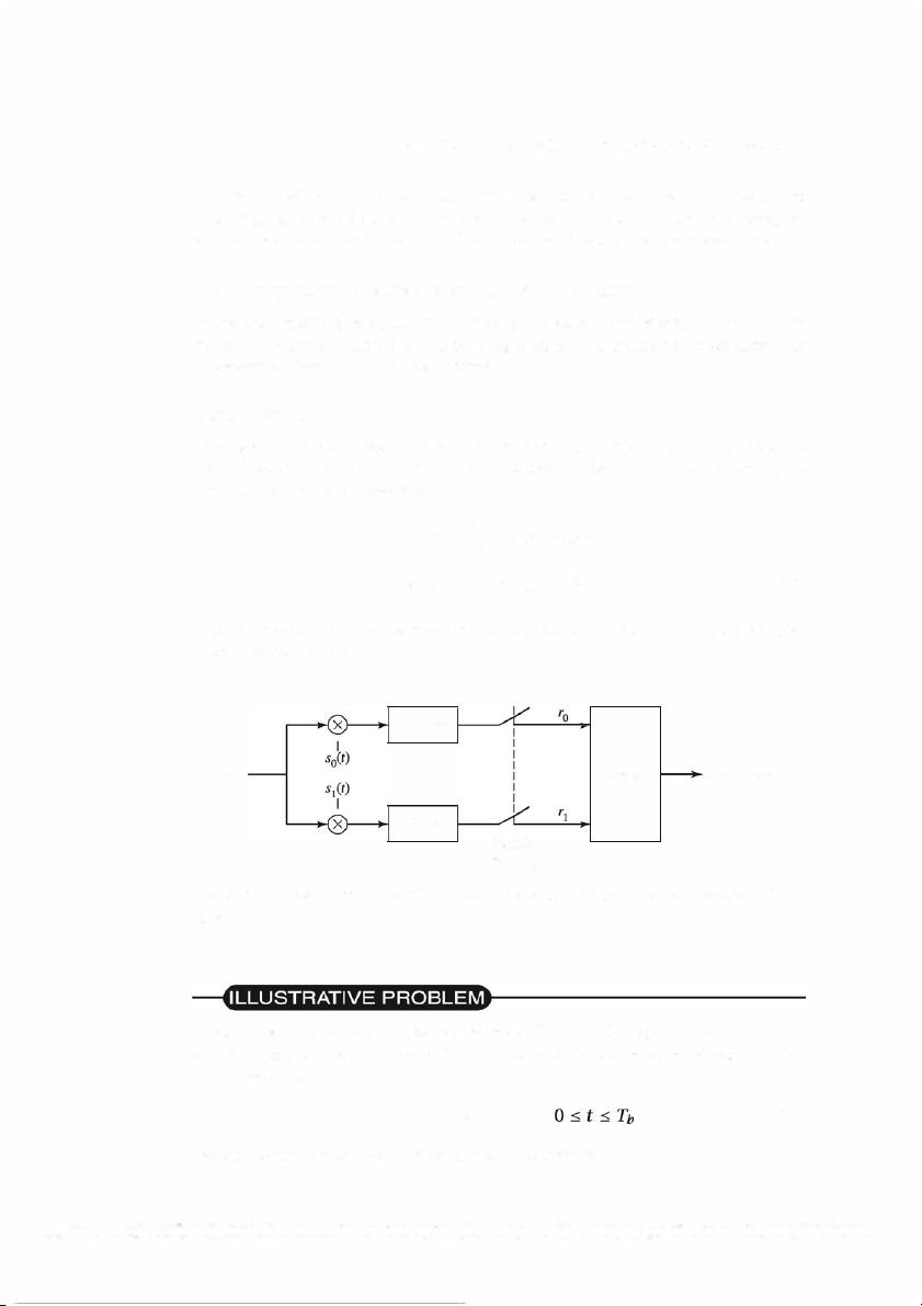
The signal correlator cross-correlates the received signal r ( t) with the two possible
transmitted signals so ( t) and si( t), as illustrated in Figure 5 .1. That is, the signal
correlator computes the two outputs ro(t) J: r(T)so(T) dT = r1 (t) f: r(T)S1 (T) dT (5.2.2) =
in the interval 0 :-:::: t :-:::: Tb, samples the two outputs at t Tb, and feeds sampled = the outputs to the detector. J�O dr: r(t) Detector Output data J�O dr: I Sample at t 1/, =
Figure 5.1: Cross-correlation of the received signal r(t) with the two transmitted sig nals
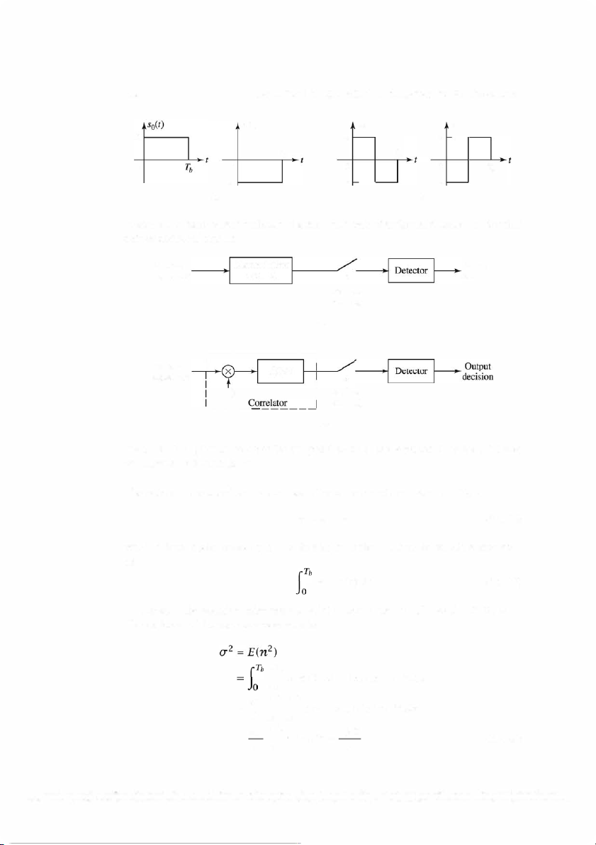
Illustrative Problem 5.1 [Signal Correlator] Suppose the signal waveforms so(t)
and si(t) are as shown in Figure 5.2, and let so(t) be the transmitted signal. Then the received signal is r(t) so(t) = + n(t), (5.2.3)
Determine the correlator outputs at the sampling instants.
Copyright 2011 Cengage Leaming. AJI Rights Reserved. May not be copied, scanned, or duplicated, in whole or in part. Due to eJectronic rights, some third party content may be suppressed from the eBook andlor eChapter(s).
Editorial review has deemed that any suppressed content does not materially affect the overall learning experience. Cengage Learning reserves the right to remove additional content at any time if subsequent rights restrictions l'«tuire it.
5.2. BINARY SIGNAL TRANSMISSION 185 s0(t) A 0 0 -A
Figure 5.2: Signal waveforms so(t) and 51 (t) for a binary communication system
When the signal r ( t) is processed by the two signal correlators shown in Figure 5 .1,
the outputs ro and r1 at the sampling instant t = Tb are ro = J :b r(t)so(t) dt = f
:b s6(t) dt + f :b n(t)so(t) dt = E+no (5.2.4) and r1 = J :b r(t)s1 (t) dt = J
:b so(t)s1 (t) dt + J :b n(t)s1 (t) dt = n1 (5.2.5)
where no and n 1 are the noise components at the output of the signal correlators; that is, no= J :b n(t)so(t) dt n1 = J :b n(t)s1 (t) dt (5.2.6)
and E = A 2 Tb is the energy of the signals so ( t) and s1 ( t) . We also note that the two
signal waveforms are orthogonal; that is, J :b so(t)s1 (t) dt = 0 (5.2.7)
On the other hand, when 51 (t) is the transmitted signal, the received signal is r (t) = s1 (t) + n(t),
It is easy to show that, in this case, the signal correlator outputs are (5.2.8)
Copyright 2011 Cengage Leaming. AJI Rights Reserved. May not be copied, scanned, or duplicated, in whole or in part. Due to eJectronic rights, some third party content may be suppressed from the eBook andlor eChapter(s).
Editorial review has deemed that any suppressed content does not materially affect the overall learning experience. Cengage Learning reserves the right to remove additional content at any time if subsequent rights restrictions l'«tuire it.
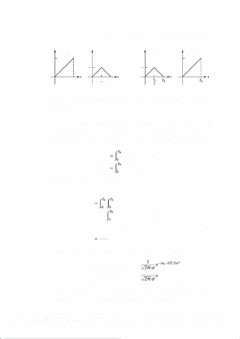
CHAPTER 5. BASEBAND DIGITAL TRANSMISSION 186 Output of Output of Output of Output of Correlator 0 Correlator 1 Correlator 0 Correlator 1 E E E E 2 2 T 0 T b b 0 Tb 0 0 (a) 2 (b)
Figure 5.3: Noise-free correlator outputs. (a) so(t) was transmitted. (b) s1 (t) was transmitted
Figure 5 .3 illustrates the two noise-free correlator outputs in the interval 0 .:-::: t .:-::: Tb for
each of the two cases-that is, when so(t) is transmitted and when s1 (t) is transmitted.
Because n(t) is a sample function of a white Gaussian process with power spec
trum No/2, the noise components no and n1 are Gaussian with zero means-that is, E(no) so(t)E [n(t)] dt = 0 E(n1) s1(t)E[n(t)] dt = 0 (5.2.9)
and variances al, for i = 1, 2, where al = E(n�) Si(t)si(T)E[n(t)n(T)] dt dT N = -f Si(t)si(T)D(t-T)dtdT = __Q T sb? (t) dt 2 f0 i (5.2.10) N, EN i = 0, 1 2 o' (5.2.11)
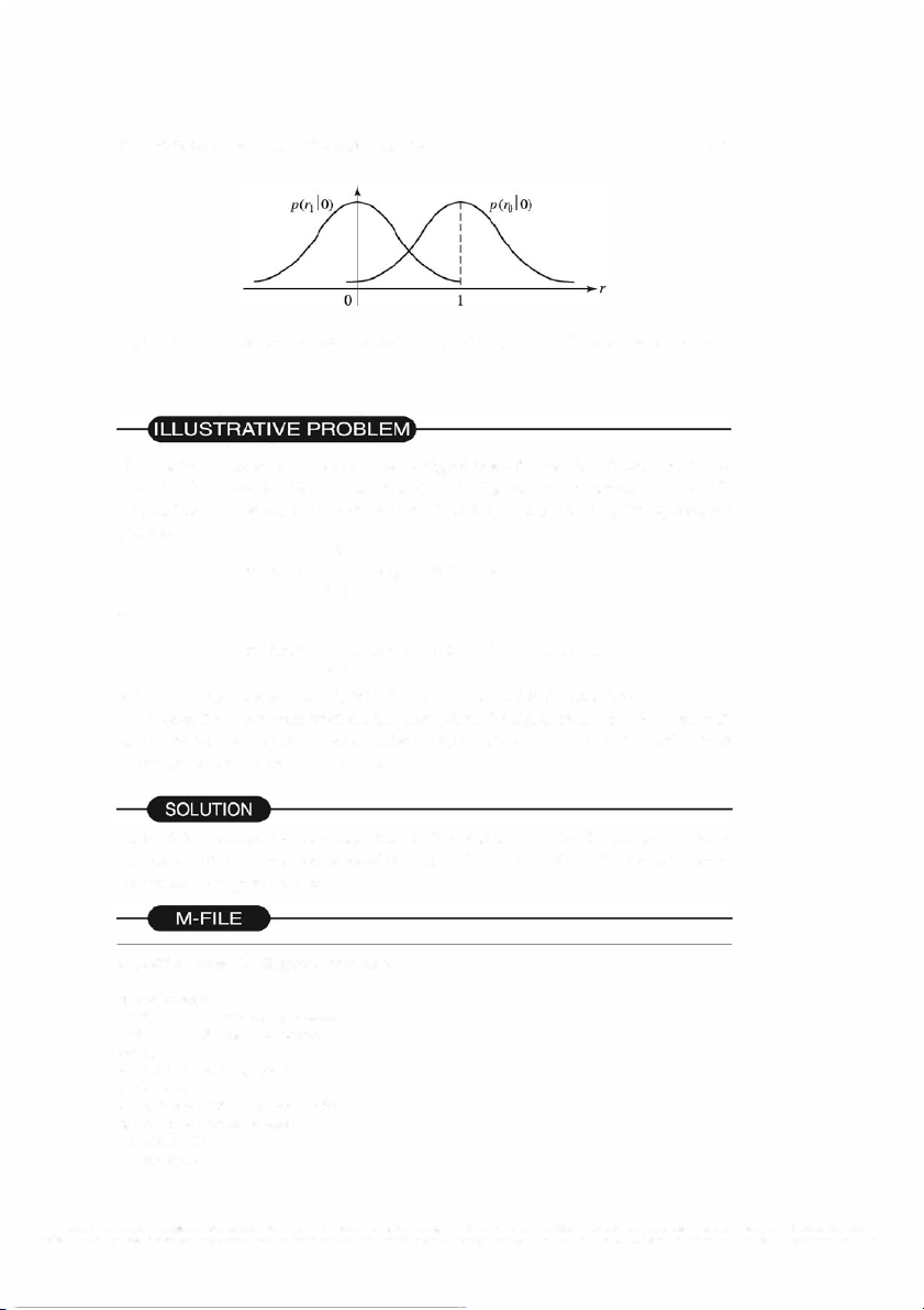
Therefore, when so ( t) is transmitted, the probability density functions of ro and r1 are
p(ro I so(t) was transmitted) = 1 -rz /2a2 = 1 p( r1 I s0( . t) d) was transm1tte (5.2.12) T ilhle u se tr a tw e o d i p n ro Fi b g a u b r i e l it 5y . 4.d en Si si mtiyl arflu y n , ct w io hens , s d1e n ( ott)e ids tarsa n p s ( mi r tt o ed , I r o 0 is) z aernod- mpea(nr 1 Ga usIs ia 0 n ), are
with variance cr2 and r1 is Gaussian with mean value E and variance cr2•
Copyright 2011 Cengage Leaming. AJI Rights Reserved. May not be copied, scanned, or duplicated, in whole or in part. Due to eJectronic rights, some third party content may be suppressed from the eBook andlor eChapter(s).
Editorial review has deemed that any suppressed content does not materially affect the overall learning experience. Cengage Learning reserves the right to remove additional content at any time if subsequent rights restrictions l'«tuire it.
5.2. BINARY SIGNAL TRANSMISSION 187
Figure 5.4: Probability density functions p(ro I 0) and p(r1 I 0) when so(t) is trans mitted
Illustrative Problem 5.2 [Correlation of Signal Waveforms] Sample the signal wave
forms in Illustrative Problem 5.1 at a rate F5 = 20/Tb (sampling interval T5 = Tb/20)
and perform the correlation of r(t) with so(t) and s1 (t) numerically; that is, compute and plot k
ro(kTs)= I r(nTs)so(nT5), k=l,2, ... ,20 n=l and k
r1(kTs)= I r(nT5)si(nT5), k=l,2, ... ,20 n=l
when (a) so(t) is transmitted signal and (b) s1 (t) is the transmitted signal.
Repeat the above computations and plots when the signal samples r(kT5) are cor
rupted by additive white Gaussian noise samples n(kT5), 1 :-s: k :-s: 20, which have zero mean and variance 2 a- = 0.1 and a-2 = 1.
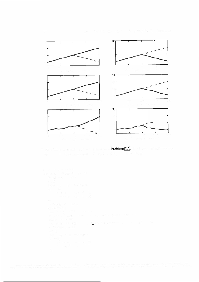
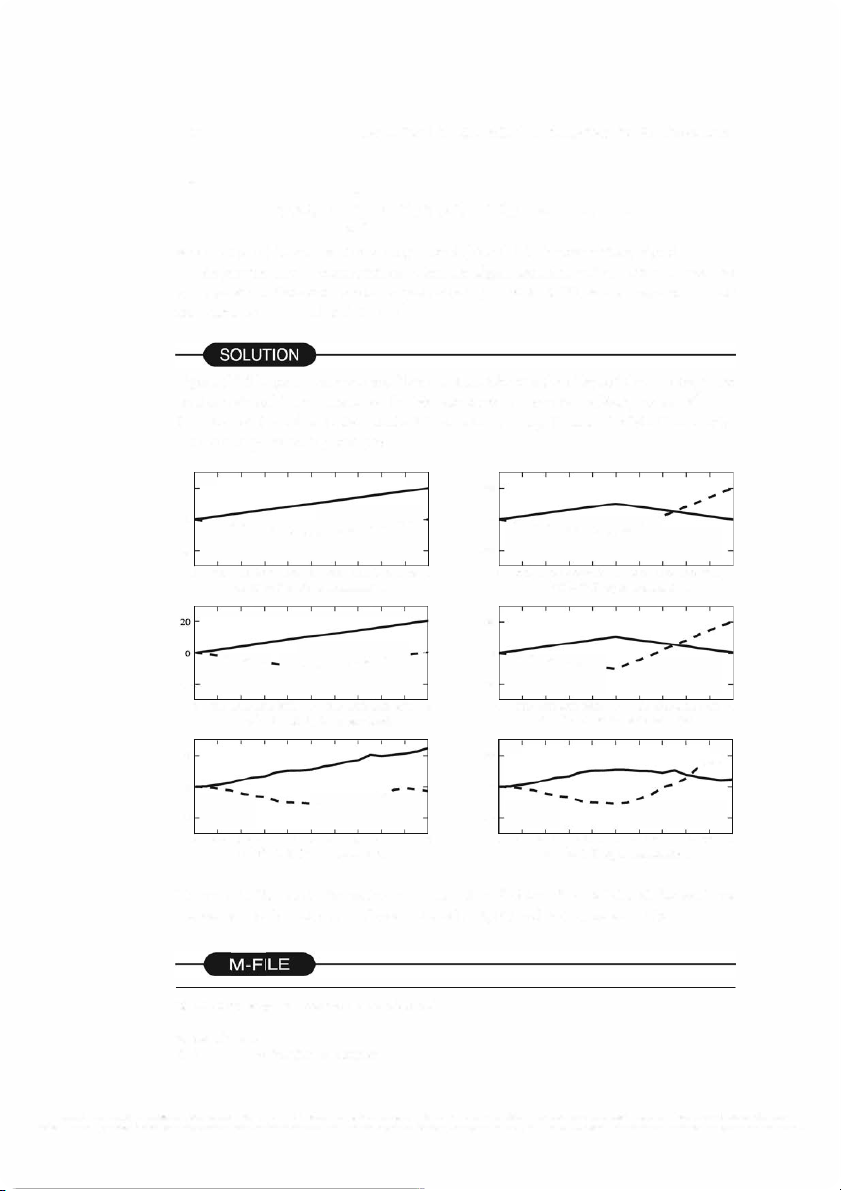
Figure 5 .5 illustrates the correlator outputs. We note the effect of the additive noise on
the outputs of the correlator, especially when 2
a- = 1. The MATLAB script for these computations is given below.
% MATLAB script for Illustrative Problem 5 .2 % Initialization: K=20; % Number of samples A=1; % Signal amplitude l=O:K; % Defining signal waveforms: s_O=A *ones(1,K);
s_ l=[A *ones(1,K/2) -A *ones(1,K/2)];
% Initializing output signals: r_O=zeros(1,K); r_l=zeros(1,K);
Copyright 2011 Cengage Leaming. AJI Rights Reserved. May not be copied, scanned, or duplicated, in whole or in part. Due to eJectronic rights, some third party content may be suppressed from the eBook andlor eChapter(s).
Editorial review has deemed that any suppressed content does not materially affect the overall learning experience. Cengage Learning reserves the right to remove additional content at any time if subsequent rights restrictions l'«tuire it. 188
CHAPTER 5. BASEBAND DIGITAL TRANSMISSION 30 20 20 10 10 0 0 20Tb 0 5Tb lOTb 15Tb 20Tb 0 5Tb lOTb 15Tb (a) cr2= 0 & S
(b) a2= 0 & S1 is transmitted 0 is transmitted 30 20 20 10 10 0 0 20Tb 0 5Tb lOTb 15Tb 20Tb 0 5Tb lOTb 15Tb ( c) <:P= 0.1 & S
(d) cr2= 0.1 & S1 is transmitted 0 is transmitted 30 20 20 10 10 --- 0 .... 0 20Tb 0 5Tb lOTb 15Tb 20Tb 0 5Tb lOTb 15Tb ( e) (f) 0 is transmitted
Figure 5.5: Correlator outputs in Illustrative Solid and dashed lines rep
resent the output of correlation with so ( t) and s1 ( t), respectively. % Case 1: noise-N(O,O) noise=random(' Normal' ,0,0, 1,K); % Sub-case s s_O: = s=s_O; r=s+noise; % received signal for n=1 :K
r_O(n)=sum(r(1 :n). *s_0(1 :n)); r_l(n)=sum(r(1 :n). *s_l (1 :n)); end % Plotting the results: subplot(3,2, 1)
plot(l,[O r_O],' -',l,[O r_l],' --')
set(gca, 'XTickLabel' ,{' 0 ',' 5Tb',' lOTb',' 15Tb', '20Tb'}) axis([O 20 -5 30])
xlabel('(a) \sigmaA2= 0 & S {O} is transmitted','fontsize',10) % Sub-case s s_J: = s=s_l; r=s+noise; % received signal for n=1 :K
r_O(n)=sum(r(1 :n).*s_0(1 :n));
r_l(n)=sum(r(1 :n).*s_l(1 :n)); end
Copyright 2011 Cengage Leaming. AJI Rights Reserved. May not be copied, scanned, or duplicated, in whole or in part. Due to eJectronic rights, some third party content may be suppressed from the eBook andlor eChapter(s).
Editorial review has deemed that any suppressed content does not materially affect the overall learning experience. Cengage Learning reserves the right to remove additional content at a
ny time if subsequent rights restrictions l'«tuire it.
5.2. BINARY SIGNAL TRANSMISSION 189 % Plotting the results: subplot(3,2,2)
plot(l,[O r_O],' -',l,[O r_l], ' --') set(gca,
'XTickLabel' ,{' 0 ', 'STb',' lOTb',' lSTb',' 20Tb'}) axis([O 20 -5 30])
xlabel('(b) \sigma"2= 0 & S_{l} is transmitted','fontsize',10) % Case 2: noise-N(0,0.1)
noise=random( 'Normal' ,0,0.1, 1,K); % Sub-case s s_O: = s=s_O; r=s+noise; % received signal for n=1 :K
r_O(n)=sum(r(1 :n).*s_Q(1 :n));
r_l(n)=sum(r(1 :n).*s_l(1 :n)); end % Plotting the results: subplot(3,2,3)
plot(l,[O r_O],' -',I,[O r_l], ' --') set(gca,
'XTickLabel' ,{' 0 ',' STb' ,' 10Tb',' lSTb', '20Tb'}) ax.is([O 20 -5 30])
xlabel('(c) \sigma"2= 0.1 & S_{O} is transmitted','fontsize',10) % Sub-case s _J: = s s=s_l; r=s+noise; % received signal for n=1 :K
r_O(n)=sum(r(1 :n).*s_0(1 :n));
r_l(n)=sum(r(1 :n).*s-1(1 :n)); end % Plotting the results: subplot(3,2,4) plot(l,[O r_O],' -',I,[O r_l], ' --') set(gca,
'XTickLabel, ,{' 0,', STb' ,' lOTb' , lSTb' , 20Tb'}) axis([O 20 -5 30])
xlabel('(d) \sigma"2= 0.1 & S_{l} is transmitted','fontsize',10) % Case 3: noise-N(O,l) noise=random( 'Normal' ,0, 1, 1,K); % Sub-case s s_O: = s=s_O; r=s+noise; % received signal for n=1 :K
r_O(n)=sum(r(1 :n).*s_0(1 :n));
r_l(n)=sum(r(1 :n).*s_l(1 :n)); end % Plotting the results: subplot(3,2,5) plot(l,[O r_O],' -',l,[O r_l],' --')
set(gca,, XTickLabel, ,{, 0,', STb, ', lOTb, ', lSTb,', 20Tb, }) axis([O 20 -5 30])
xlabel('(e) \sigma"2= 1 & S_{O} is transmitted','fontsize',10) % Sub-case s _J: = s s=s_l; r=s+noise; % received signal for n=1 :K
r_O(n)=sum(r(1 :n).*s_0(1 :n));
r_l(n)=sum(r(1 :n).*s_l(1 :n));
Copyright 2011 Cengage Leaming. AJI Rights Reserved. May not be copied, scanned, or duplicated, in whole or in part. Due to eJectronic rights, some third party content may be suppressed from the eBook andlor eChapter(s).
Editorial review has deemed that any suppressed content does not materially affect the overall learning experience. Cengage Learning reserves the right to remove additional content at any time if subsequent rights restrictions l'«tuire it. 190
CHAPTER 5. BASEBAND DIGITAL TRANSMISSION end % Plotting the results: subplot(3,2,6)
plot(l,[O r_O],' -',l,[O r_l], ' --')
set(gca, 'XTickLabel' ,{' 0 ',' 5Tb',' lOTb',' 15Tb',' 20Tb'}) axis([O 20 -5 30])
xlabel('(f) \sigrnaA2= 1 & S_{l} is transrnitted','fontsize',10) Matched Filter
The matched filter provides an alternative to the signal correlator for demodulating
the received signal r(t). A filter that is matched to the signal waveform s(t), where
0 :s: t :s: Tb, has an impulse response h(t) s(Tb - t), (5.2.13) =
Consequently, the signal waveform-say, y ( t) -at the output of the matched filter
when the input waveform is s(t) is given by the convolution integral f: (5.2.14) y (t) S(T)h(t - T) dT =
If we substitute in (5.2.14) for h(t - T) from (5.2.13), we obtain f: S(T)s(Tb - t (5.2.15) y(t) + T) dT =
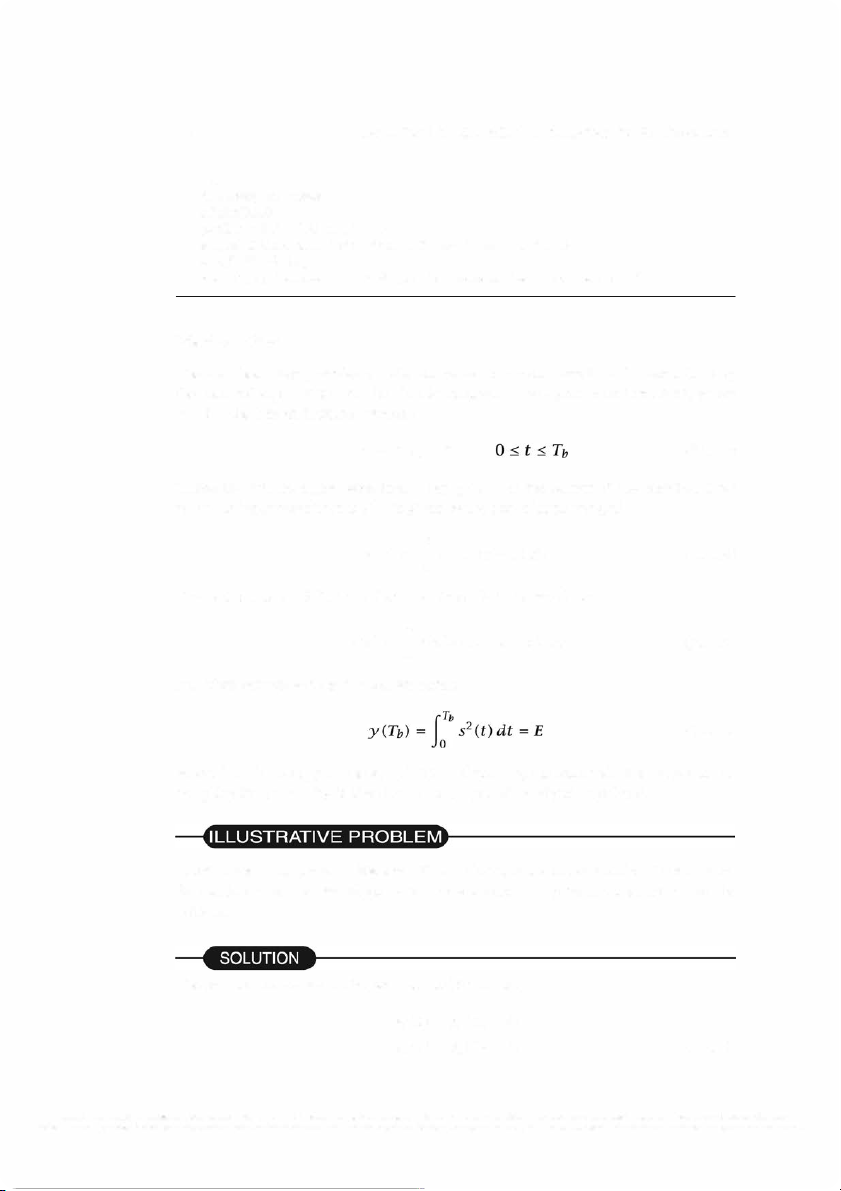
and if we sample y (t) at t Tb, obtain = we (5.2.16)
where E is the energy of the signal s ( t). Therefore, the matched filter output at the
sampling instant t Tb is identical to the output of the signal correlator. =
Illustrative Problem 5.3 [Matched Filter] Consider the use of matched filters for the
demodulation of the two signal waveforms shown in Figure 5 .2 and determine the outputs.
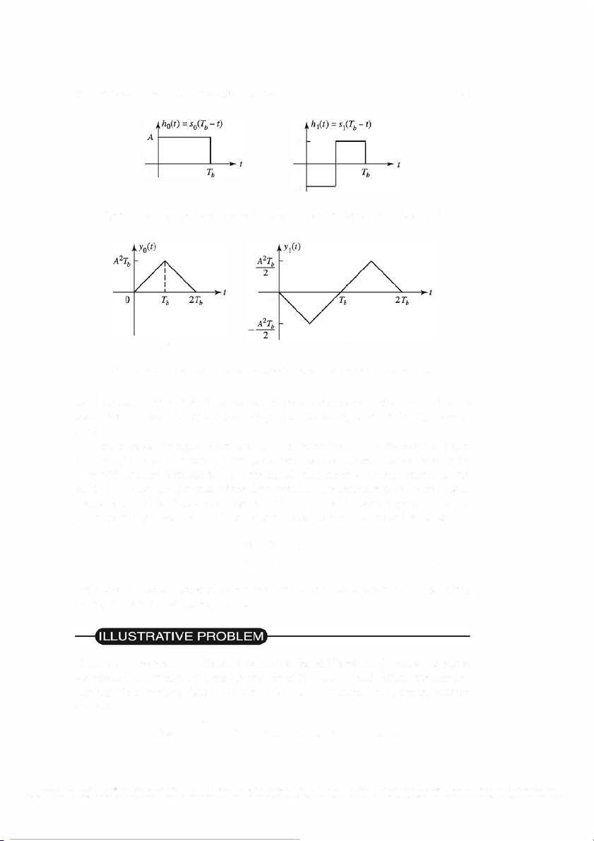
The impulse responses of the two matched filters are ho(t) so(Tb - t) = h1(t) s1(Tb - t) (5.2.17) =
Copyright 2011 Cengage Leaming. AJI Rights Reserved. May not be copied, scanned, or duplicated, in whole or in part. Due to eJectronic rights, some third party content may be suppressed from the eBook andlor eChapter(s).
Editorial review has deemed that any suppressed content does not materially affect the overall learning experience. Cengage Learning reserves the right to remove additional content at any time if subsequent rights restrictions l'«tuire it.
5.2. BINARY SIGNAL TRANSMISSION 191 A 0 0 -A
Figure 5 .6: Impulse responses of matched filters for signals so ( t) and s1 ( t) 0 (a) (b)
Figure 5 .7: Signal outputs of matched filters when so ( t) is transmitted
as illustrated in Figure 5.6. Note that each impulse response is obtained by folding the
signal s ( t) to obtain s ( -t) and then delaying the folded signal s ( -t) by Tb to obtain s(Tb -t).
Now suppose the signal waveform so(t) is transmitted. Then the received signal r ( t) = so ( t) +
n ( t) is passed through the two matched filters. The response of the
filter with impulse response ho ( t) to the signal component so ( t) is illustrated in Fig
ure 5.7(a). Also, the response of the filter with impulse response h1 (t) to the signal
component so(t) is illustrated in Figure 5.7(b). Hence, at the sampling instant t = Tb,
the outputs of the two matched filters with impulse responses ho ( t) and hi ( t) are ro = E +no r1 = n1 (5.2.18)
respectively. Note that these outputs are identical to the outputs obtained from sampling
the signal correlator outputs at t = Tb.
Illustrative Problem 5.4 [Match Filtering of Signal Waveforms] Sample the signal
waveform in Illustrative Problem 5 .3 at a rate of F5 = 20 I Tb and perform the matched
filtering of the received signal r ( t) with so ( t) and s1 ( t) numerically; that is, compute and plot k
Yo(kTs) = L r(nTs)so(kTs -nTs), k= 1,2, ... ,20 n=l
Copyright 2011 Cengage Leaming. AJI Rights Reserved. May not be copied, scanned, or duplicated, in whole or in part. Due to eJectronic rights, some third party content may be suppressed from the eBook andlor eChapter(s).
Editorial review has deemed that any suppressed content does not materially affect the overall learning experience. Cengage Learning reserves the right to remove additional content at any time if subsequent rights restrictions l'«tuire it. 192
CHAPTER 5. BASEBAND DIGITAL TRANSMISSION and k
Y1(kTs) = L r(nTs)si(kTs-nTs), k= 1,2, ... ,20 n=l
when (a) so ( t) is the transmitted signal and (b) s1 ( t) is the transmitted signal.
Repeat the above computations when the signal samples r(kT5) are corrupted by
additive white Gaussian noise samples n(kT5), 1 ::5: k ::5: 20, which have zero mean
and variance cr2 = 0.1 and cr2 = 1.
Figure 5 .8 illustrates the matched filter outputs. We note the effect of the additive noise
on the matched filter outputs for the two variances of the noise. Clearly, when cr2 = 1,
the effect of the noise on the matched filter outputs is significant. The MATLAB script
for the computation is given next 20 2a a a - , - -- , ------- ------ --- _, -20 -20
a 5Th lOTh 15Th 20Th a 5Th lOTh 15Th 2aTu a
a 5Th lOTh 15Th 20Th a 5Th lOTh 1 5Th 20Th a
(a) cr2= 0 & Sa is transmitted
(b) o2= 0 & S1 is transmitted 20 --- a -- --- - --- -- --- -2a -2a
a 5Th 1 aTu 15Th 2aTu a 5Th 1 aTu 15Th 2aTu a
a 5Th JaTu 15Th 2aTu a STh lOTh ISTh 2aTu a
(c) cr2= 0.1 & Sa is transmitted
(d) o2= 0.1 & S1 is transmitted 2a 2a ,. - a .,,,,. a - - - ,,, -2a -2a
a 5Th lOTh 15Th 20Th a 5Th IaTu 15Th 2aTu a
a STh IOTh 15Th 20Th a STb IOTb 1 5Th 2aTu a
(e) o2= l & S0 is transmitted
(t) o2= 1 & S1 is transmitted
Figure 5.8: Matched filter outputs in Illustrative Problem 5.4. Solid and dashed lines
correspond to the outputs of filters matched to so ( t) and s1 ( t), respectively.
% MATLAB script for Illustrative Problem 5.4. % Initialization: K=20; % Number of samples
Copyright 2011 Cengage Leaming. AJI Rights Reserved. May not be copied, scanned, or duplicated, in whole or in part. Due to eJectronic rights, some third party content may be suppressed from the eBook andlor eChapter(s).
Editorial review has deemed that any suppressed content does not materially affect the overall learning experience. Cengage Learning reserves the right to remove additional content at any time if subsequent rights restrictions l'«tuire it.
5.2. BINARY SIGNAL TRANSMISSION 193 A=1; % Signal amplitude l=O:K; % Defining signal waveforms: s_O=A *ones(1,K);
s_l=[A*ones(1,K/2) -A*ones(1,K/2)];
% Initializing output signals: y_O=zeros(1,K); y_l=zeros(1,K); % Case 1: noise-N(O,O)
noise=random( 'Normal' ,0,0, 1,K); % Sub-case s = s_O: s=s-0; y=s+noise; % received signal y_O=conv(y,wrev(s_O)); y _ l=conv(y,wrev(s_ l)); % Plotting the results: subplot(3,2, 1)
plot(l,[O y_0(1 :K)], '-k' ,l,[O y_l(1 :K)],' --k')
set(gca, 'XTickLabel' ,{' 0 ', 'STb',' lOTb',' lSTb',' 20Tb'}) axis([O 20 -30 30])
xlabel('(a) \sigmaA2= 0 & S {O} is transmitted','fontsize',10) % Sub-case s _J: = s s=s_l; y=s+noise; % received signal y _O=conv(y,wrev(s_O)); y _l=conv(y,wrev(s_ l)); % Plotting the results: subplot(3,2,2)
plot(l,[O y_0(1 :K)],' -k' ,l,[O y_l(1 :K)],' --k')
set(gca, 'XTickLabel' ,{' 0 ',' STb' ,' 10Tb',' 15Tb', '20Tb'}) axis([O 20 -30 30])
xlabel('(b) \sigmaA2= 0 & S_{l} is transmitted','fontsize',10) % Case 2: noise-N(0,0.1)
noise=random( 'Normal' ,0,0.1, 1,K); % Sub-case s = s_O: s=s-0; y=s+noise; % received signal y _O=conv(y ,wrev(s_O)); y _l=conv(y ,wrev(s_ l)); % Plotting the results: subplot(3,2,3)
plot(l,[O y_0(1 :K)],' -k' ,l,[O y_l(1 :K)],' --k')
set(gca, 'XTickLabel, ,{' 0,', STb' ,' 10Tb' , lSTb' , 20Tb'}) axis([O 20 -30 30])
xlabel('(c) \sigmaA2= 0.1 & S_{O} is transmitted','fontsize',10) % Sub-case s _J: = s s=s_l; y=s+noise; % received signal y _O=conv(y ,wrev(s_O)); y _l=conv(y,wrev(s_ l)); % Plotting the results: subplot(3,2,4)
plot(l,[O y_0(1 :K)],' -k' ,l,[O y_l(1 :K)],' --k')
set(gca, 'XTickLabel' ,{' 0 ',' STb' ,' 10Tb',' lSTb', '20Tb'})
Copyright 2011 Cengage Leaming. AJI Rights Reserved. May not be copied, scanned, or duplicated, in whole or in part. Due to eJectronic rights, some third party content may be suppressed from the eBook andlor eChapter(s).
Editorial review has deemed that any suppressed content does not materially affect the overall learning experience. Cengage Learning reserves the right to remove additional content at any time if subsequent rights restrictions l'«tuire it. 194
CHAPTER 5. BASEBAND DIGITAL TRANSMISSION axis([O 20 -30 30])
xlabel('(d) \sigrna"2= 0.1 & S_{l} is transrnitted','fontsize',10} % Case 3: noise-N(O,l)
noise=random(' Normal' ,0, 1, 1,K); % Sub-case s s_O: = s=s_O; y=s+noise; % received signal y _O=conv(y ,wrev(s_O)); y_l=conv(y,wrev(s_ l)}; % Plotting the results: subplot(3,2,5) plot(l,[O y_0(1 :K}],' -k' ,l,[O y_l(1 :K}],' --k'}
set(gca, 'XTickLabel' ,{' 0 ',' 5Tb',' lOTb',' 15Tb',' 20Tb'}) axis([O 20 -30 30])
xlabel('(e) \sigrna"2= 1 & S {O} is transrnitted','fontsize',10) % Sub-case s s_J: = s=s_l; y=s+noise; % received signal y _O=conv(y, wrev(s_O)}; y_ l=conv(y,wrev(s_ l)); % Plotting the results: subplot(3,2,6) plot(l,[O y_0(1 :K)],' -k' ,l,[O y_l(1 :K)],' --k')
set(gca, 'XTickLabel' ,{' 0 ',' 5Tb',' lOTb',' 15Tb',' 20Tb'}) axis([O 20 -30 30])
xlabel('(f) \sigrna"2= 1 & S_{l} is transrnitted','fontsize',10) The Detector
The detector observes the correlator or matched filter outputs ro and r1 and decides
on whether the transmitted signal waveform is so ( t) or s1 ( t) , which correspond to the
transmission of either a 0 or a 1, respectively. The optimum detector is defined as the
detector that minimizes the probability of error.
Illustrative Problem 5.5 [Binary Detection] Let us consider the detector for the sig
nals shown in Figure 5.2, which are equally probable and have equal energies. The
optimum detector for these signals compares ro and r1 and decides that a 0 was trans
mitted when ro > r1 and that a 1 was transmitted when r1 > ro. Determine the probability of error.
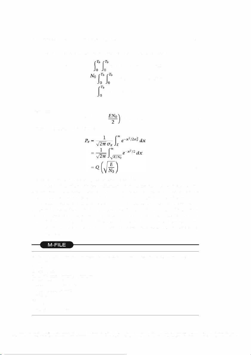
When s0(t) is the transmitted signal waveform, the probability of error is Pe P( r1 o) P(n1 o) P(n1 = > r = > E +n = - no > E) (5.2.19)
Because n1 and no are zero-mean Gaussian random variables, their difference x
ni - no is also zero-mean Gaussian. The variance of the random variable xis (5.2.20)
Copyright 2011 Cengage Leaming. AJI Rights Reserved. May not be copied, scanned, or duplicated, in whole or in part. Due to eJectronic rights, some third party content may be suppressed from the eBook andlor eChapter(s).
Editorial review has deemed that any suppressed content does not materially affect the overall learning experience. Cengage Learning reserves the right to remove additional content at any time if subsequent rights restrictions l'«tuire it.
5.2. BINARY SIGNAL TRANSMISSION 195
But E(n1no) 0 because the signal waveforms are orthogonal; that is, = E(n1 no) E so(t)s1 (T)n(t)n(T) dt dT = 2 So(t)s1 (T)O(t - T) dt dT = No = T so(t)s1 (t) dt 0 (5.2.21) = Therefore, E(x2) ( 2 ENo u� (5.2.22) = = =
Hence, the probability of error is (5.2.23)
The ratio EI No is called the signal-to-noise ratio (SNR).
The derivation of the detector performance given in the example was based on the
transmission of the signal waveform so ( t). The reader may verify that the probability
of error that is obtained when s1 ( t) is transmitted is identical to that obtained when
so (t) is transmitted. Because the O's and 1 's in the data sequence are equally probable,
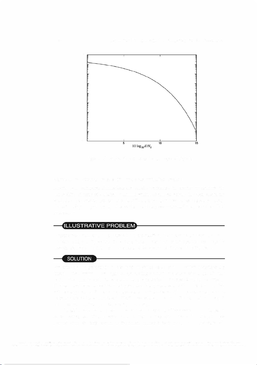
the average probability of error is that given by (5.2.23). This expression for the prob
ability of error is evaluated by using the MATLAB script given next and is plotted in
Figure 5 .9 as a function of the SNR, where the SNR is displayed on a logarithmic scale
( 10 log 10 EI No). As expected, the probability of error decreases exponentially as the SNR increases.
% The MATLAB script that generates the probability of error versus the signal-to-noise ratio. initiaLsnr=O; finaLsnr=15; snr_step=0.25;
snr_in_dB=initiaLsnr:snr_step:final_snr; for i=1 :length(snr_in_dB), snr=1 DA (snr_in_dB(i)/1 O); Pe(i)=Qfunct(sqrt(snr)); echo off; end; echo on; semilogy( snr _in_dB ,Pe);
Copyright 2011 Cengage Leaming. AJI Rights Reserved. May not be copied, scanned, or duplicated, in whole or in part. Due to eJectronic rights, some third party content may be suppressed from the eBook andlor eChapter(s).
Editorial review has deemed that any suppressed content does not materially affect the overall learning experience. Cengage Learning reserves the right to remove additional content at any time if subsequent rights restrictions l'«tuire it. 196
CHAPTER 5. BASEBAND DIGITAL TRANSMISSION 10° 10-1 10-2 10-3 10-4 10-5 10-6 10-7 10-8 10-9 0
Figure 5.9: Probability of error for orthogonal signals
Monte Carlo Simulation of a Binary Communication System
Monte Carlo computer simulations are usually performed in practice to estimate the
probability of error of a digital communication system, especially in cases where the
analysis of the detector performance is difficult to perform. We demonstrate t he method
for estimating the probability of error for the binary communication system described previously.
Illustrative Problem 5.6 [Monte Carlo Simulation] Use Monte Carlo simulation to
estimate and plot Pe versus SNR for a binary communication system that employs
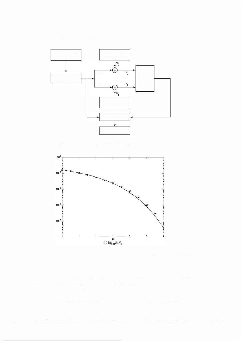
correlators or matched filters. The model of the system is illustrated in Figure 5.10.
We simulate the generation of the random variables ro and r1, which constitute the
input to the detector. We begin by generating a binary sequence of O's and 1 's that
occur with equal probability and are mutually statistically independent. To accomplish
this task, we use a random number generator that generates a uniform random number
with a range ( 0, 1). If the number generated is in the range ( 0, 0. 5), the binary source
output is a 0. Otherwise, it is a 1. If a 0 is generated, then ro E + no and r1 n1. If = =
a 1 is generated, then ro no and r1 E n = = + i.
The additive noise components no and n 1 are generated by means of two Gaussian
noise generators. Their means are zero, and their variances are 2 a ENo/2. For =
convenience, we may normalize the signal energy E to unity (£ 1) and vary 2 = a •
Copyright 2011 Cengage Leaming. AJI Rights Reserved. May not be copied, scanned, or duplicated, in whole or in part. Due to eJectronic rights, some third party content may be suppressed from the eBook andlor eChapter(s).
Editorial review has deemed that any suppressed content does not materially affect the overall learning experience. Cengage Learning reserves the right to remove additional content at any time if subsequent rights restrictions l'«tuire it.
5.2. BINARY SIGNAL TRANSMISSION 197 Uniform random Gaussian random number generator number generator 0/E Output Binary data Detector data source 1/E Gaussian random number generator Compare Error counter
Figure 5.10: Simulation model for Illustrative Problem 5.6 10-s 0 2 4 8 10 12
Figure 5 .11: Error probability from Monte Carlo simulation compared with theoretical
error probability for orthogonal signaling
Note that the SNR, which is defined as E/No, is then equal to l/2u2• The detector
output is compared with the binary transmitted sequence, and an error counter is used
to count the number of bit errors.
Figure 5 .11 illustrates the results of this simulation for the transmission of N =
10, 000 bits at several different values of SNR. Note the agreement between the
Copyright 2011 Cengage Leaming. AJI Rights Reserved. May not be copied, scanned, or duplicated, in whole or in part. Due to eJectronic rights, some third party content may be suppressed from the eBook andlor eChapter(s).
Editorial review has deemed that any suppressed content does not materially affect the overall learning experience. Cengage Learning reserves the right to remove additional content at any time if subsequent rights restrictions l'«tuire it. 198
CHAPTER 5. BASEBAND DIGITAL TRANSMISSION
simulation results and the theoretical value of Pe given by (5.2.23). We should also
note that a simulation of N = 10,000 data bits allows us to estimate the error probabil ity reliably down to about Pe 10-3. In other words, with N = = 10,000 data bits, we
should have at least ten errors for a reliable estimate of Pe. MATLAB scripts for this problem are given next.
% MATLAB script for Illustrative Problem 5.6. echo on SNRindB1=0:1 :12; SNRindB2=0:0.1 :12; for i=1 :length(SNRindBl), % simulated error rate
smld_err_prb(i)=smldPe54(SNRindB 1 (i)); echo off ; end; echo on ; for i=1 :length(SNRindB2),
SNR=exp(SNRindB2(i)*log(10)/1 O); % theoretical error rate
theo_err_prb(i)=Qfunct(sqrt(SNR)); echo off ; end; echo on; % Plotting commands follow.
semilogy(SNRindBl,smld_err_prb,' * '); hold
semilogy(SNRindB2,theo_err_prb);
function [p]=smldPe54(snr_in_dB) % [p]=smldPe54(snr_in....dB) %
SMWPE54 finds the probability of error for the given %
snr .Jn....dB, signal-to-noise ratio in dB. E=1; SNR=exp(snLin_dB*log(10)/10); % signal-to-noise ratio sgma=E/sqrt(2*SNR);
% sigma, standard deviation of noise N=10000;
% generation of the binary data source for i=1 :N, temp=rand;
% a uniform random variable over (0,1) if (temp<0.5), dsource(i)=O;
% With probability 112, source output is 0. else dsource(i)=1;
% With probability 112, source output is 1. end end;
% detection, and probability of error calculation numoferr=O; for i=1 :N,
Copyright 2011 Cengage Leaming. AJI Rights Reserved. May not be copied, scanned, or duplicated, in whole or in part. Due to eJectronic rights, some third party content may be suppressed from the eBook andlor eChapter(s).
Editorial review has deemed that any suppressed content does not materially affect the overall learning experience. Cengage Learning reserves the right to remove additional content at any time if subsequent rights restrictions l'«tuire it.
5.2. BINARY SIGNAL TRANSMISSION 199 % matched filter outputs if (dsource(i)==O), rO=E+gngauss(sgma); rl=gngauss(sgma); % if the source output is "O" else rO=gngauss(sgma); rl=E+gngauss(sgma);
% if the source output is "1 " end; % Detector follows. if (rO>rl), decis=O; % Decision is "O". else decis=1; % Decision is "l ". end; if (decis-=dsource(i)),
% If it is an error, increase the error counter. numoferr=numoferr+ 1 ; end; end; p=numoferr/N;
% probability of error estimate
In Figure 5.11, simulation and theoretical results completely agree at low signal-to
noise ratios, whereas at higher SNRs they agree less. Can you explain why? How
should we change the simulation process to result in better agreement at higher signal to-noise ratios? 5.2.2
Other Binary Signal Transmission Methods
The binary signal transmission method described above was based on the use of orthog
onal signals. Next, we describe two other methods for transmitting binary information
through a communication channel. One method employs antipodal signals. The other
method employs an on-off-type signal.
Antipodal Signals for Binary Signal Transmission
Two signal waveforms are said to be antipodal if one signal waveform is the negative
of the other. For example, one pair of antipodal signals is illustrated in Figure 5.12(a).
A second pair is illustrated in Figure 5.12(b).
Suppose we use antipodal signal waveforms so(t) = s(t) and 51 (t) = -s(t) to
transmit binary information, where s ( t) is some arbitrary waveform having energy E.
The received signal waveform from an AWGN channel may be expressed as r(t) = ±s(t) + n(t), (5.2.24)
The optimum receiver for recovering the binary information employs a single correlator
or a single matched filter matched to s ( t), followed by a detector, as illustrated in
Figure 5.13. Let us suppose that s(t) was transmitted, so that the received signal is r(t) = s(t) + n(t) (5.2.25) from
Copyright 2011 Cengage Leaming. AJI Rights Reserved. May not be copied, scanned, or duplicated, in whole or in part. Due to eJectronic rights, some third party content may be suppressed the eBook andlor eChapter(s).
Editorial review has deemed that any suppressed content does not materially affect the overall learning experience. Cengage Learning reserves the right to remove additional content at any time if subsequent rights restrictions l'«tuire it. 200
CHAPTER 5. BASEBAND DIGITAL TRANSMISSION s1(t) s0(t) s1(t) A A A Tb Tb 0 0 0 0 Tb -A -A -A (a) (b)
Figure 5 .12: Examples of antipodal signals. (a) A pair of antipodal signals. (b) Another pair of antipodal signals Received Matched filter Output . . · s1gn 1 a r( t) s (T.b t) d _ t ec1s1on Sample at t T,, = (a) 1-----------1 Received I signal r(t) f.o'Odt t I s(t) I Sample at t T,, = _____ (b)
Figure 5.13: Optimum receiver for antipodal signals. (a) Matched filter demodulator. (b) Correlator demodulator
The output of the correlator or matched filter at the sampling instant t = Tb is r=E+n (5.2.26)
where E is the signal energy and n is the additive noise component, which is expressed as n = n(t)s(t) dt (5.2.27)
Because the additive noise process n(t) is zero mean, it follows that E(n) = 0.
The variance of the noise component n is 0 f Tb E [n(t)n(T)] s(t)s(T) dt dT N f Tb fTb
= T 0 0 <5(t - T)S(t)S(T) dt dT = No f T 0 b s2(t) dt = NoE (5.2.28) 2 2
Copyright 2011 Cengage Leaming. AJI Rights Reserved. May not be copied, scanned, or duplicated, in whole or in part. Due to eJectronic rights, some third party content may be suppressed from the eBook andlor eChapter(s).
Editorial review has deemed that any suppressed content does not materially affect the overall learning experience. Cengage Learning reserves the right to remove additional content at any time if subsequent rights restrictions l'«tuire it.
5.2. BINARY SIGNAL TRANSMISSION 201 -E E
Figure 5 .14: Probability density functions for the input to the detector
Consequently, the probability density function of r when s(t) is transmitted is 1 p(r I s(t) was transmitted) e-(r-£J2 /20-2 (5.2.29) = p(r I 0) = J2IT (J
Similarly, when the signal waveform -s(t) is transmitted, the input to the detector is r = -E + n (5.2.30)
and the probability density function of r is 1 - (r+£)2 /2a2
p(r I -s(t) was transmitted) = p(r I 1) = u e (5 .2.31) J2IT
These two probability density functions are illustrated in Figure 5.14.
For equally probable signal waveforms, the optimum detector compares r with the
threshold zero. If r > 0, the decision is made that s(t) was transmitted. If r < 0, the
decision is made that -s(t) was transmitted. The noise that corrupts the signal causes
errors at the detector. The probability of a detector error is easily computed. Suppose
that s(t) was transmitted. Then the probability of error is equal to the probability that r < 0; that is, Pe= P(r < 0) 1 f o = e-(r-E)z 120-2 dr J2IT (J -00 = 1 f-E/a e-r 12 2 d - - r J2IT -00 = Q = Q(ffeo) (5.2.32)
A similar result is obtained when -s(t) is transmitted. Consequently, when the
two signal waveforms are equally probable, the average probability of error is given by (5.2.32).
When we compare the probability of error for antipodal signals with that for or
thogonal signals given by (5.2.23), we observe that, for the same transmitted signal
energy E, antipodal signals result in better performance. Alternatively, we may say
Copyright 2011 Cengage Leaming. AJI Rights Reserved. May not be copied, scanned, or duplicated, in whole or in part. Due to eJectronic rights, some third party content may be suppressed from the eBook andlor eChapter(s).
Editorial review has deemed that any suppressed content does not materially affect the overall learning experience. Cengage Learning reserves the right to remove additional content at any time if subsequent rights restrictions l'«tuire it. 202
CHAPTER 5. BASEBAND DIGITAL TRANSMISSION
that antipodal signals yield the same performance (same error probability) as orthogo
nal signals by using one-half of the transmitted energy of orthogonal signals. Hence,
antipodal signals are 3 dB more efficient than orthogonal signals.
Illustrative Problem 5.7 [Correlation of Antipodal Signal Waveforms] In antipo
dal signaling, the signal waveform so(t) is defined as so(t) = A, 0:::::; t:::::; Tb
and zero otherwise. The received signal is r(t) = ±so (t) + n(t). Sample the received
signal r(t) and so(t) at the rate F5 = 20/Tb and perform the correlation of r(t) with
so(t) numerically; that is, compute and plot k
ro(kTs) = L r(nT5)so(nT5), k = 1,2, ... ,20 n=l
when (a) so(t) is the transmitted signal and (b) -so(t) is the transmitted signal. Per
form the computations when the additive noise is Gaussian having zero mean and vari ances 2 2 2 a = 0, a = 0.1, and a = 1.
Figure 5.15 illustrates the correlator outputs for different noise variances. The MAT
LAB script for the computation is given next
% MATLAB script for Illustrative Problem 5.7. % Initialization: K=20; % Number of samples A=1; % Signal amplitude l=O:K;
s_O=A *ones(1,K);% Signal waveform
r_O=zeros(1,K); % Output signal % Case 1: noise-N(O,O)
noise=random( 'Normal' ,0,0, 1,K}; % Sub-case s = s_O: s=s_O; r=s+noise; % received signal for n=1 :K
r_O(n)=sum(r(1 :n). *s_0(1 :n)); end % Plotting the results: subplot(3,2, 1) plot(l, [O r_O])
set(gca, 'XTickLabel' ,{' 0 ',' 5Tb',' lOTb',' 15Tb', '20Tb'})
Copyright 2011 Cengage Leaming. AJI Rights Reserved. May not be copied, scanned, or duplicated, in whole or in part. Due to eJectronic rights, some third party content may be suppressed from the eBook andlor eChapter(s).
Editorial review has deemed that any suppressed content does not materially affect the overall learning experience. Cengage Learning reserves the right to remove additional content at any time if subsequent rights restrictions l'«tuire it.
