Homework 5 Môn Inventory Management | Trường Đại học Quốc tế, Đại học Quốc gia Thành phố Hồ Chí Minh

lOMoAR cPSD| 58605085
School of Industrial Engineering & Management (IEM) Inventory Management
International University, VNU-HCM
Instructor: Dr. Nguyen Van Hop Homework 5_ Chapter 5
Deadline: Class Day next week I.
Problem Statement: Managing Class A Items 1. Fast – moving items A:
- Assumptions: Items are A categories, fast moving. Demand is probabilistic, normally distributed
- Given: Economic data (holding cost, carrying rate, ordering cost, unit variable cost),
demand distribution and its parameters, lead time, cost of each shortage (B1) (for (Q,s)
model) , fraction of cost per unit short at the end of each period (B3), review time R (for (R,s ,S) model)
- Decision variables: Order quantity Q, reorder point s
- Method: Continuous review: Reorder point – Order quantity (Q,s) model, Reorder point –
Order – up – to level (s,S) model using simultaneous parameter selection (iterative
procedure), Periodic review – Reorder point – Order up to level (R,s ,S) using revised power approximation method 2. Slow – moving items A
- Assumption: Two types: very slow – moving, expensive times (using Q=1¿ and slow –
moving items (Q>1¿. For very slowing moving items, assume demand distribution is
Poisson, D<0.0763∗v, lead time is constant, backorder consideration. For slow moving
items, it is the same as in (Q,s) model.
- Given: For Base stock model: Demand rate, unit variable cost, carrying rate r, fraction
charge per unit charge (B2),
- Decision variables: For base stock model: reorder point s. For (Q,s) model: Order quantity
Q and reorder point s
- Method: Base stock model (For Q=1), Continuous review: Order quantity – Reorder point
(Q,s) ( For Q>1) II. Homework
Problem 1: Fast moving items A (Q,s) system (Problem 8.1-page 349 textbook)
Consider an (Q,s) system of control for a single item and with normally distributed forecast errors.
For the following example develop order quantity Q, safety stock factor k and the associated total
relevant costs per year for two strategies:
1. Q=EOQ and corresponding k
2. Simultaneous best (Q,k) pair Item characteristics:
Ordering cost A=$5, carrying rate r=0.16/ yr, unit cost v=$ 2 per unit, demand rate
D=1000units per year, σL=80units, expected number of stockout occasions per year being
N=0.5 per year, fixed cost per stockout occasion B1=$50 lOMoAR cPSD| 58605085
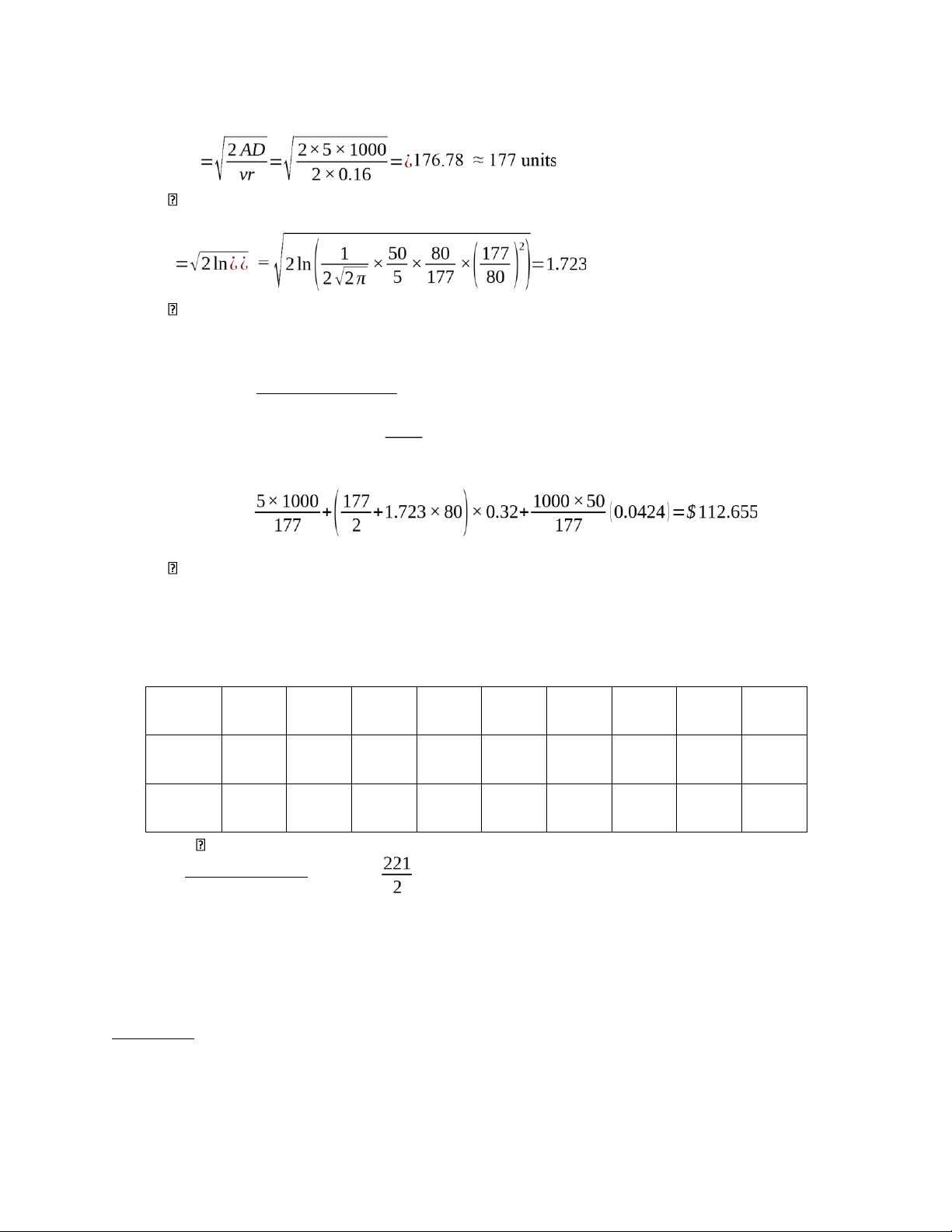
1. Q = EOQ and corresponding k EOQ
Q=EOQ=177units k k = 1.723 Total cost: AD Q DB1 TC (Q,k )= +( +kδL)h+ Pr ( X ≥k ) Q 2 Q ¿ Total cost is $112.655
2. Simultaneous best (Q,k) pair
We have: EOQ = 177 units. With the iteration procedure, we obtain: Iteratio 1 2 3 4 5 6 7 8 n 9
176.7 211.0 218.6 220.3 220.7 220.8 220.8 220.8 220.8 Q 8 1 5 8 8 7 9 9 9
1.722 1.616 1.594 1.589 1.588 1.588 1.587 1.587 1.587 k 6 5 4 4 3 0 9 9 9
Q = 220.89 ≈ 221 units , k = 1.5879
5×10001000×50 The total cost =
+(+1.5879×80)×0.32+ (0.056 ) ¿ $111.304 221221
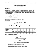
Problem 2: (Q,s) system (Problem 8.3-page 350 textbook) lOMoAR cPSD| 58605085
Ceiling Drug is concerned about the inventory control of an important item. Currently they are
using an (Q,s) system where Q is the EOQ and the safety stock factor k is selected based on a B2
v shortage costing method. Relevant parameter values are estimated to be:
Demand rate D=2500units per year, unit variable cost v=$ 10 perunit, ordering cost A=$5,
carrying rate r=0.25 $/$/year, fractional charge per unit short B2=$0.6, mean demand during lead
time x^L=500units, lead time demand standard deviation σL=100units.
a. What are the Q and s values currently in use?
b. Determine the simultaneous best value of Q and s.
c. What is the percent penalty (in the total of replenishment, carrying, and shortage costs) of
the simpler sequential approach?
Hint: Decision rule for a specified fractional charge (B2) (Section 7.7.6 – page 263 textbook) Qr
a. Select k so as to satisfy pu≥(k )=D B2
b. Reformulate Total cost with B2 derivative function of Q = 0 formular of Q
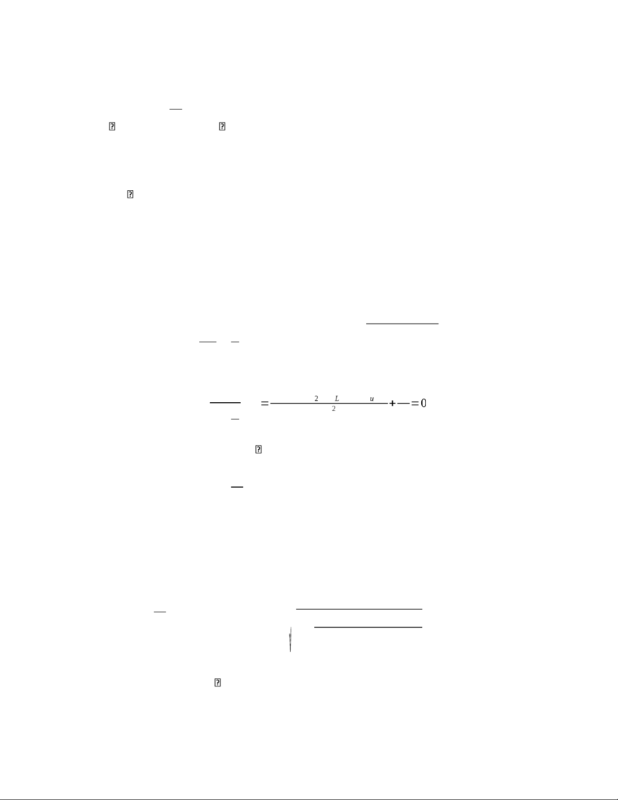
Total cost TC= ADQ +(Q2 +k σ ) L vr+
B2 v σLQGu (k ) D, where the shortage cost term is D
composed of the ESPRC, σLGu (k), the number of cycles per year Q , and the cost per unit short vB2
Gu(k): a special function of the unit normal (mean 0 and std dev 1) variable used to find
the expected shortages per replenishment cycle (ESPRC) (can be obtained from k, by
using a table lookup shown in appendix II), k is as part (a)
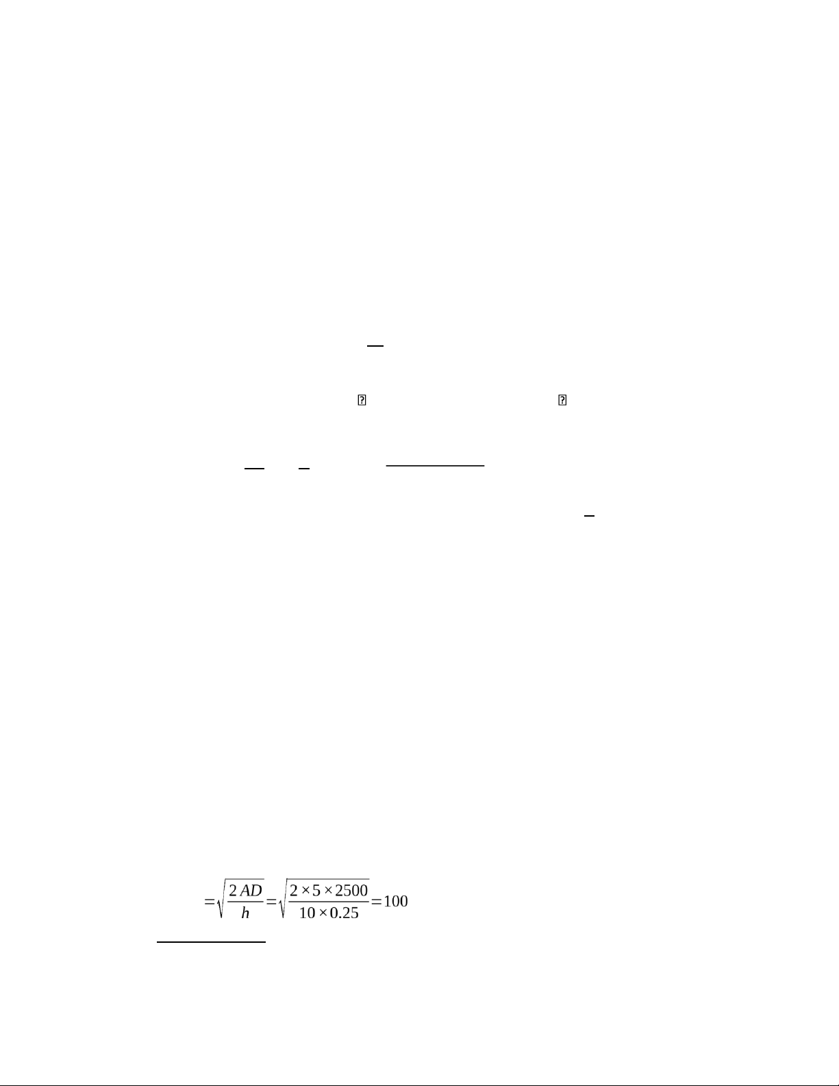
c. Sequencing approach means that the procedure in which Q = EOQ calculation, then k is calculated with respect to Q D = 2500 units/year v = $10 per unit A = $5 r = 0.25$/$/year B2 = $0.6 x^L = 500 units σL = 100 units a. Q=EOQ units Qr 100×0.25 = = 0.0167 lOMoAR cPSD| 58605085 DB2 2500×0.6 Qr
pu≥(k )=D B2 =0.0167 k = 2.12 The reorder point:
s = x^L+σLk=500+100×2.12=712units
The (Q, s) currently in use is (100, 712) b. We have: Total cost :
ETRC(k ,Q)= AD +(Q+k σ ) L
vr+B2 v σLGu (k ) D Q 2 Q
Take derivative of both sides: dETRC (k )
−AD+B v σ D×G (k ) vr dQ Q 2 Qr
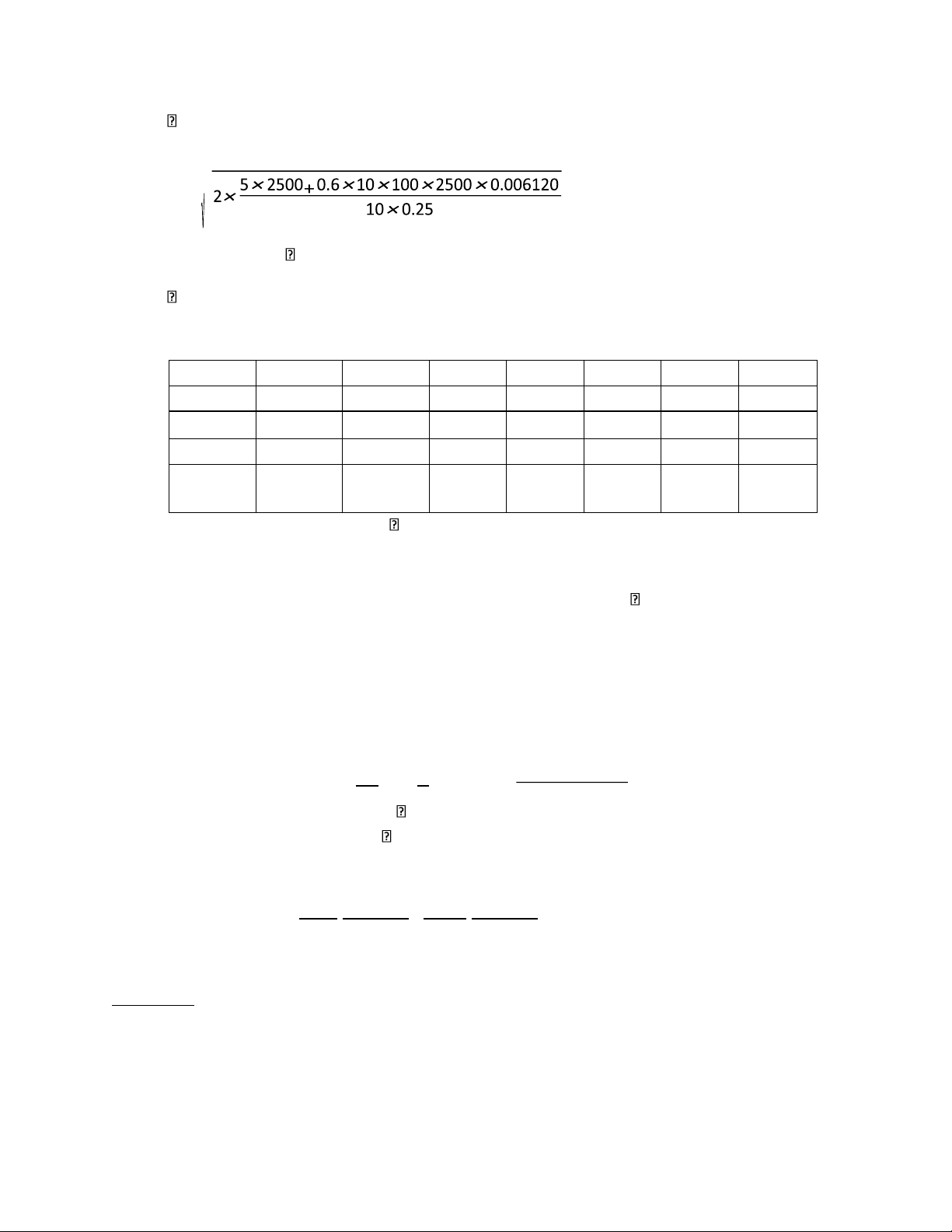
Also, we have: pu≥(k )=D B2 Q = EOQ = 100 units o Iteration 1: Q = EOQ = 100 units Qr
Q = 2× AD+B2 v σLD×Gu (k) vr
pu≥(k )=D B2 =0.0167 k = 2.12 lOMoAR cPSD| 58605085
Gu (k )=0.006120 o Iteration 2: Q = = 131.697
pu≥(k )=0.02195 k = 2.02
Gu (k )=0.008046
With the iteration procedure, we obtain: Iteration 1 2 3 4 5 6 7 Q 100
131.697 140.197 143.057 144.043 145.043 145.04 pu≥(k ) 0.0167
0.02195 0.02337 0.02384 0.02401 0.02417 0.02417 k 2.12 2.02 1.99 1.98 1.97 1.97 1.97 G 0.008046 u (k) 0.00612 0.00872 0.00896 0.0092 0.0092 0.0092 0
Q = 145 units and k = 1.97 The reorder point:
s = x^L+σLk=500+100×1.97=697units The
(Q, s) currently in use is (145, 697)
c. We have the formula of total cost:
ETRC(Q,k)= ADQ +(Q2 +k σ ) L vr+
B2 v σLQGu (k) D ETRC(100, 2.12) = $871.8
ETRC (145, 1.97) = $855.13 The percent penalty:
ETRC(100,2.12)−ETRC (145,1.97) PCP =
×100=0.0195×100=1.95% ETRC(145,1.97)
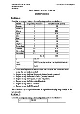
Problem 3: Fast moving items (R,s,S) system (Problem 8.7-page 350 textbook)
a. Consider an item for which an (R,s ,S) system is used. The review interval is 1 week.
Other characteristics include lead time L=2weeks, demand rate D=800units/ yr,
ordering cost A=$20, unit cost v=$ 1.50 per unit, carrying rate r=0.26$/$/year, lOMoAR cPSD| 58605085
fractional charge per unit short per time B3=0.3 $/$/short/week, variance during
replenishment interval σR+L=14.2units.
Using the revised power approximation, find the appropriate values of s and S. (Assume that
there are exactly 52 weeks per year)
b. Repeat for another item with the same characteristics except v=$ 150 per unit. L = 2 weeks = year, R = 1 week = year a. x^R units x^R units QP units z sp units Q 250 Also: . x^R 15 s¿ sp=48units
S = sp+QP=298units b. x^R units x^R units
QP=1.3×(15)0.494 × unit s z sp units Q 28 Also, we have: . x^R 15 lOMoAR cPSD| 58605085
s=sp=69units
S = sp+QP=97units
Problem 4: Slow moving item – Base stock policy
Consider the case of a high-value item with unit cost v=$ 350 perunit, demand rate D=25units
per year, carrying rate r=0.24 $/$/year, lead time L=3.5 weeks=3.5/52 year, ordering cost
A=$3.20. and fraction charge per unit short B2 is estimated to be 1/5 i.e., 350/5 or $70 per unit
backordered). Assume the system employs the policy of ordering one-for-one each time a
demand drops to a specific inventory position (order quantity Q=1¿ Develop the policy (find the inventory position) We have: Q = 1
Pr ( X=S+1) r 0.24 = = =0.048/units Pr ( X≤ s+1) D B Mean demand: 3.5
x^L=DL=25( 52 )=1.68units Pr(X=S+1) . 1,0.0048 /units Pr(X ≤s+1)
POISSON . DIST(s+1,0.0048,TRUE)
Using Excel s = 4 or S = 5. Therefore, the order point is 4 units