Khái niệm chính và tiến trình | Cơ học lượng tử | Trường Đại học Khoa học Tự nhiên, Đại học Quốc gia Hà Nội

PHYS20101
Introduction to Quantum Mechanics
SUMMARY OF IMPORTANT CONCEPTS
The following is a summary originally prepared by A C
Phillips, adapted by G D Lafferty, A J Bray and W R Flavell QUANTUM WAVEFUNCTIONS
• Particle and wave properties are described by a wavefunction Ψ which
ebbs and flows in accordance with the time-dependent Schrödinger equation (TDSE), ˆ ∂Ψ H Ψ = ih ∂t where ˆ
H is the ‘energy operator’, usually called the Hamiltonian operator.
• Ψ 2 is a probability density for position. In one dimension, 2 P(x x
, t)dx = Ψ( ,t) dx = the probability of finding the particle at time t x dx between and x +
• If you look everywhere, you will be certain to find the particle. Ψ is
normalised at all times t such that, integrated over all space, the
probability of finding the particle is unity. In one dimension: +∞ ∫ Ψ 2
(x, t) dx = 1 −∞ 1 QUANTUM STATES
Wavefunctions represent the possible states of motion of real particles.
They bear only a passing resemblance to the well-defined particle
trajectories encountered in classical physics, and are called quantum states (QS).
• A QS provides precise predictions for the probabilities of the results of measurements.
• In the absence of measurements, a QS evolves deterministically in
accordance with the time-dependent Schrödinger equation.
• Any linear superposition of solutions of the TDSE is also a solution.
(This is not true of superpositions of solutions of the time-independent
Schrödinger equation (TISE) unless they have the same energy, i.e. they are degenerate.)
• A QS is fragile. A measurement destroys it and replaces it by a new
quantum state which is compatible with the outcome of the measurement.
• However, we still do not understand the link between the statistical
nature of some of the predictions of quantum mechanics and the
certainties we measure in the macroscopic world. QUANTUM EVOLUTION
• Time evolution is governed by the TDSE ˆ ∂Ψ H Ψ = ih . ∂t
• If the QS is a state of certain energy E, then
Ψ = ψ e−iEt /h , where ψ satisfies the TISE ˆ H ψ = Eψ , 2
and all observable properties are constant in time, Such a state is called a stationary state.
• If the QS is a state of uncertain energy with normalised wavefunction given by Ψ = t / h t / h
c ψ e−iE1
+ c ψ e−iE2 , 1 1 2 2
an energy measurement results in E with probability |c |2 or E with 1 1 2
probability |c |2, and observable properties oscillate with a period 2 2πh / E − E . 2 1
Thus if the QS is a state of uncertain energy ΔE, the timescale (δt) for
change of observable properties is of the order
δt • ΔE ≈ h .
QUANTUM MECHANICAL TUNNELLING
• If a quantum particle is subject to a confining potential V, there is a
finite probability of finding the particle in classically forbidden
regions (where E) unless the confining potential is infinite.
• A particle may thus ‘tunnel’ through a thin barrier of thickness a with
2m(V − E )
a tunnelling probability that depends upon e−2βa, where β = . h
Hence the wavefunction decays exponentially in the classically forbidden barrier region. QUANTUM OBSERVABLES
A measurable quantity or observable, A, is represented in quantum mechanics by an operator ˆ A .
In general, the outcome of a measurement of A is uncertain:
• For a system in the state Ψ(x,t), the expectation value of A is ∞
A = ∫ Ψ * (x,t) ˆ
A Ψ(x, t)dx −∞ 3
• The expectation value of A2 is ∞
A2 = ∫ Ψ * (x,t) ˆ
A 2 Ψ(x,t)dx −∞
• The uncertainty in the outcome is Δ 2 A = A2 − A
Sometimes the outcome is certain:
• If the quantum state is an eigenstate of ˆ A , Ψ = ψ where ˆ A ψ = A ψ , n n n n
the outcome is equal to the eigenvalue A . n QUANTUM COMPATIBILITY
When are observables A and B compatible?
• Physically, if we can know both precisely at the same time.
• Mathematically, if the commutator ˆ A
[ , ˆ B ] is zero, so that there exists a
complete set of QS’s with certain values for both A and B. Examples
• Position and momentum are incompatible because ˆ [x ] , ˆ p = ih
• The x and y components of angular momentum are incompatible because ˆ L , ˆ L [ ]= ihˆ L x y z 4
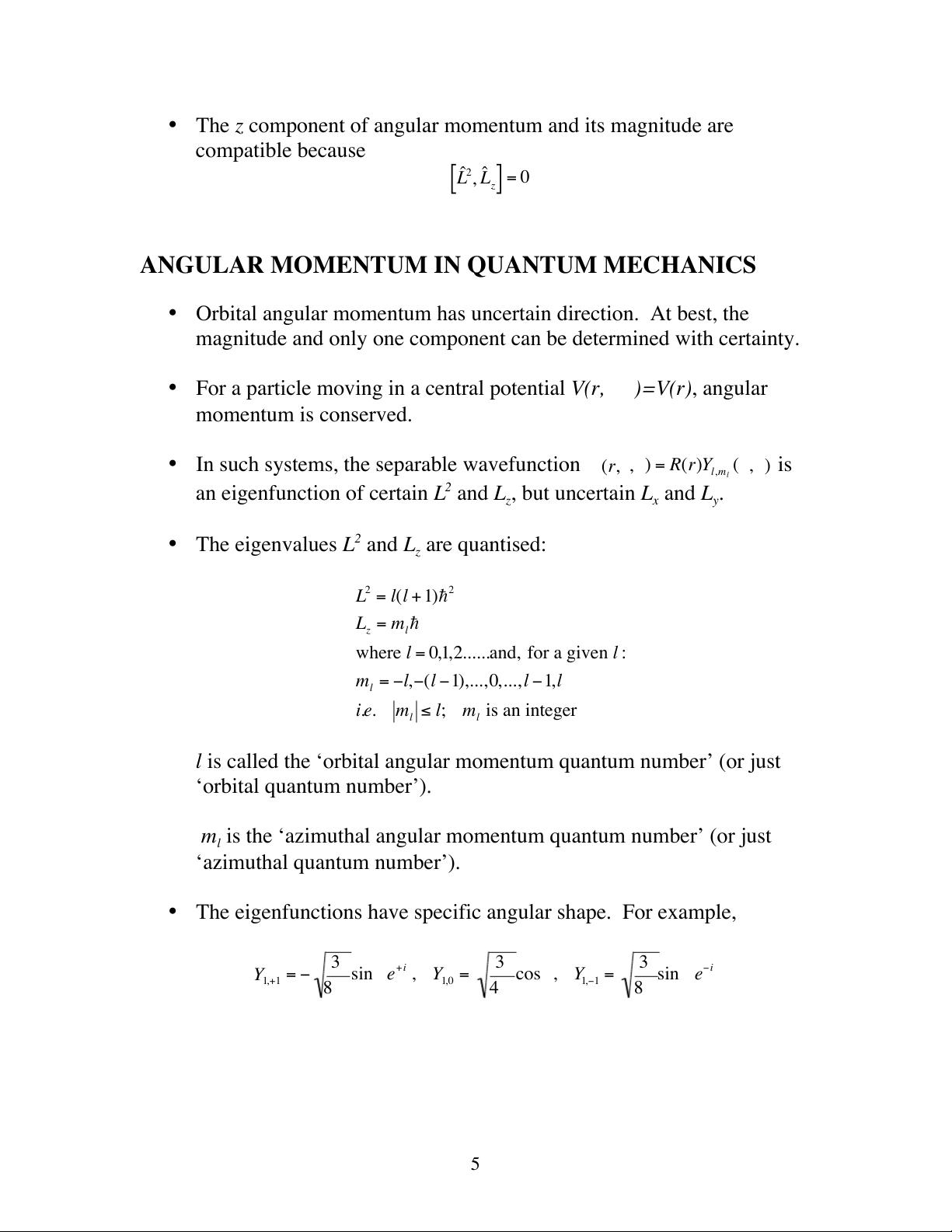
• The z component of angular momentum and its magnitude are compatible because ˆ L 2, ˆ L [ ] = 0 z
ANGULAR MOMENTUM IN QUANTUM MECHANICS
• Orbital angular momentum has uncertain direction. At best, the
magnitude and only one component can be determined with certainty.
• For a particle moving in a central potential V(r,θ,φ)=V(r), angular momentum is conserved.
• In such systems, the separable wavefunction ψ(r,θ, φ) = R(r)Y (θ,φ) is l ,ml
an eigenfunction of certain L2 and L , but uncertain L and L . z x y
• The eigenvalues L2 and L are quantised: z
L2 = l(l + 1)h2 L = m h z l
where l = 0,1,2......and, for a given l :
m = −l,−(l −1),...,0,...,l −1,l l i.e.
m ≤ l; m is an integer l l
l is called the ‘orbital angular momentum quantum number’ (or just ‘orbital quantum number’).
m is the ‘azimuthal angular momentum quantum number’ (or just l
‘azimuthal quantum number’).
• The eigenfunctions have specific angular shape. For example, 3 3 3 Y = −
sin θ e+iφ, Y = cos θ, Y = sin θ e−iφ 1,+1 8 1,0 1,−1 π 4π 8π 5
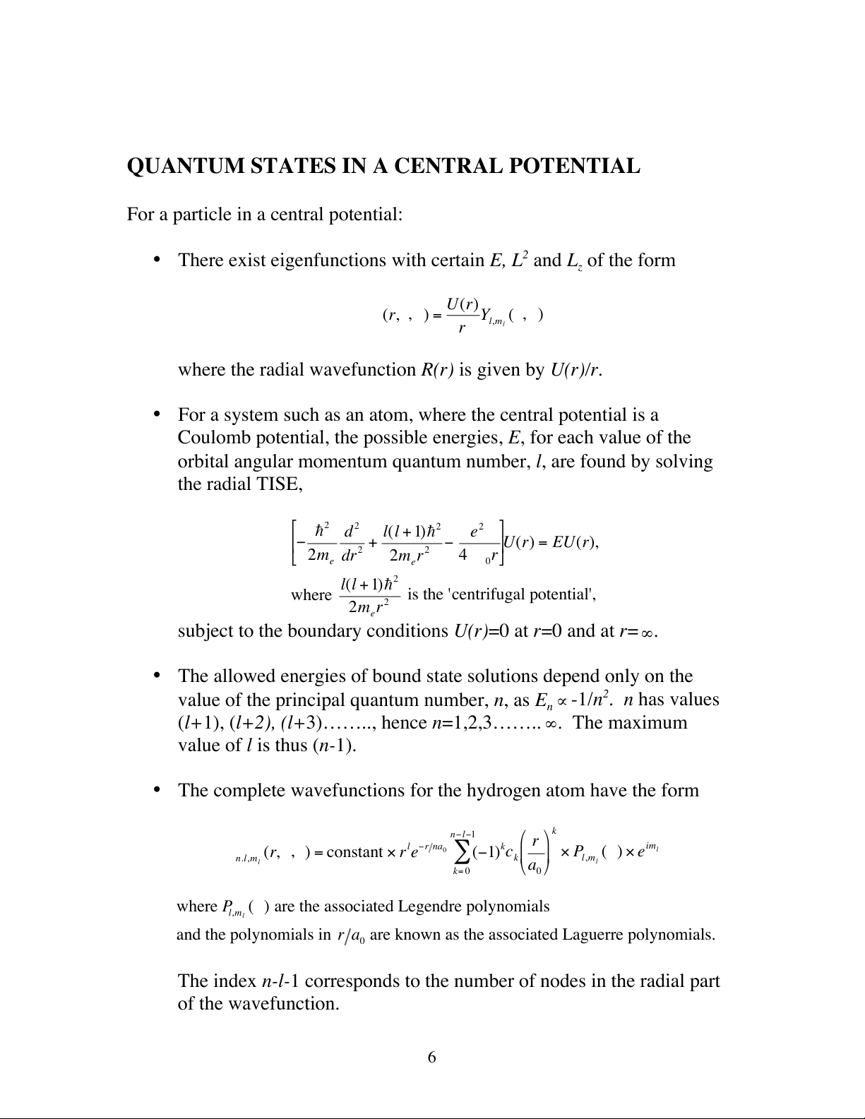
QUANTUM STATES IN A CENTRAL POTENTIAL
For a particle in a central potential:
• There exist eigenfunctions with certain E, L2 and L of the form z U(r) ψ(r,θ, φ) = Y (θ,φ) l r ,ml
where the radial wavefunction R(r) is given by U(r)/r.
• For a system such as an atom, where the central potential is a
Coulomb potential, the possible energies, E, for each value of the
orbital angular momentum quantum number, l, are found by solving the radial TISE,  h2 d2 l(l + 1)h2 e2  −  + −
 U(r) = EU(r),  2m dr2 2m r2 4πε r e e 0 l(l + 1)h2 where
is the 'centrifugal potential', r2 2me
subject to the boundary conditions U(r)=0 at r=0 and at r= ∞.
• The allowed energies of bound state solutions depend only on the
value of the principal quantum number, n, as En ∝ -1/n2. n has values
(l+1), (l+2), (l+3)…….., hence n=1,2,3…….. ∞. The maximum
value of l is thus (n-1).
• The complete wavefunctions for the hydrogen atom have the form n − l− k 1  r  ψ
(r,θ,φ) = constant × rle−r na0 ∑(−1)kc   × P (θ) × eimlφ n .l,m k l ,m l a   l k= 0 0 where P
(θ) are the associated Legendre polynomials l,ml
and the polynomials in r a are known as the associated Laguerre polynomials. 0
The index n-l-1 corresponds to the number of nodes in the radial part of the wavefunction. 6