Labor Productivity and Comparative Advantage - Bussiness ( BUS123) | Đại học Hoa Sen

C H A P T E R 3 Labor Productivity and Comparative Advantage: TheRicardian Model
Countries engage in international trade for two basic reasons, each of which
contributes to their gains from trade. First, countries trade because they are d
er. Nations, like individuals, can benefit from their differ-
ences by reaching an arrangement in which y . Second, countries . That
is, if each country produces only a limited range of goods, it can produce each of
these goods at a larger scale and hence
ly than if it tried to produce
everything. In the real world, patterns of international trade reflect the interaction
of both these motives. As a first step toward understanding the causes and effects
of trade, however, it is useful to look at simplified models in which only one of these motives is present.
The next four chapters develop tools to help us to s b give r
between them and why this trade is mutually
beneficial. The essential concept in this analysis is that of c e.
Although comparative advantage is a simple concept, experience shows that it
is a surprisingly hard concept for many people to understand (or accept). Indeed,
the late Paul Samuelson—the Nobel laureate economist who did much to develop
the models of international trade discussed in Chapters 4 and 5—once described
comparative advantage as the best example he knows of an economic principle
that is undeniably true yet not obvious to intelligent people.
In this chapter, we begin with a general introduction to the concept of com-
parative advantage and then proceed to develop a specific model of how com-
parative advantage determines the pattern of international trade. LEARNING GOALS
After reading this chapter, you will be able to: ■ ■
Explain how the Ricardian model, the most basic model of international
trade, works and how it illustrates the principle of comparative advantage. 52
CHAPTER 3■Labor Productivity and Comparative Advantage: TheRicardian Model 53 ■ ■
Demonstrate gains from trade and refute common fallacies about interna- tional trade. ■ ■
Describe the empirical evidence that wages reflect productivity and that
trade patterns reflect relative productivity.
On Valentine’s Day, 1996, which happened to fall less than a week before the crucial
February 20 primary in New Hampshire, Republican presidential candidate Patrick
Buchanan stopped at a nursery to buy a dozen roses for his wife. He took the occasion
to make a speech denouncing the growing imports of flowers into the United States,
which he claimed were putting American flower growers out of business. And it is
indeed true that a growing share of the market for winter roses in the United States is
supplied by imports flown in from South American countries, Colombia in particular. But is that a bad thing?
The case of winter roses offers an excellent example of the reasons why interna-
tional trade can be beneficial. Consider first how hard it is to supply American sweet-
hearts with fresh roses in February. The flowers must be grown in heated greenhouses,
at great expense in terms of energy, capital investment, and other scarce resources.
Those resources could be used to produce other goods. Inevitably, there is a trade-
off. In order to produce winter roses, the U.S. economy must produce fewer of other
things, such as computers. Economists use the term to describe such
The opportunity cost of roses in terms of computers is the number of
computers that could have been produced with the resources used to produce a given number of roses.
Suppose, for example, that the United States currently grows for
sale on Valentine’s Day and that the resources used to grow those roses could have produced instead. Then the n r
rs. (Conversely, if the computers were produced instead, the
opportunity cost of those 100,000 computers would be 10 million roses.)
Those 10 million Valentine’s Day roses could instead have been grown in Colombia.
It seems extremely likely that the opportunity cost of those roses in terms of comput-
ers would be less than it would be in the United States. For one thing, it is a lot easier
to grow February roses in the Southern Hemisphere, where it is summer in February
rather than winter. Furthermore, Colombian workers are less efficient than their U.S.
counterparts at making sophisticated goods such as computers, which means that a
given amount of resources used in computer production yields fewer computers in
Colombia than in the United States. So the trade-off in Colombia might be something
like 10 million winter roses for only 30,000 computers. This ffers the
. Let the United States stop growing winter roses
and devote the resources this frees up to producing computers; meanwhile, let Colom-
bia grow those roses instead, shifting the necessary resources out of its computer indus-
try. The resulting changes in production would look like Table 3-1.
Look what has happened: The world is producing just as many roses as before,
but it is now producing more computers. So this rearrangement of production, with
the United States concentrating on computers and Colombia concentrating on roses,
increases the size of the world’s economic pie. Because the world as a whole is produc-
ing more, it is possible in principle to raise everyone’s standard of living. 54
PART ONE■International Trade Theory TABLE 3-1
Hypothetical Changes in Production Million Roses Thousand Computers United States - 10 + 100 Colombia + 10 - 30 Total 0 + 70
The reason that international trade produces this increase in world output is that it allows each country to A country has a
e in producing a good if
In this example, Colombia has a comparative advantage in winter roses and the
United States has a comparative advantage in computers. The standard of living can
be increased in both places if Colombia produces roses for the U.S. market, while the
United States produces computers for the Colombian market. We therefore have an
essential insight about comparative advantage and international trade: es if e e.
This is a statement about possibilities—not about what will actually happen. In the
real world, there is no central authority deciding which country should produce roses
and which should produce computers. Nor is there anyone handing out roses and
computers to consumers in both places. Instead, international production and trade
are determined in the marketplace, where supply and demand rule. Is there any reason
to suppose that the potential for mutual gains from trade will be realized? Will the
United States and Colombia actually end up producing the goods in which each has
a comparative advantage? Will the trade between them actually make both countries better off ?
To answer these questions, we must be much more explicit in our analysis. In this
chapter, we will develop a model of international trade originally proposed by British
economist David Ricardo, who introduced the concept of comparative advantage in
the early 19th century.1 This approach, in which , is known as the . A One-Factor Economy
To introduce the role of comparative advantage in determining the pattern of interna-
tional trade, we begin by imagining that we are dealing with an economy—which we call Home—that
n. (In Chapter 4 we extend the analysis
to models in which there are several factors.) We imagine that s, and c
se, are produced. The technology of Home’s economy can be summarized by
labor productivity in each industry, expressed in terms of the , the
r required to produce a pound of cheese or a gallon of
wine. For example, it might require and
. Notice, by the way, that we’re defining unit
labor requirements as the inverse of productivity—the more cheese or wine a worker
1The classic reference is David Ricardo, The Principles of Political Economy and Taxation, first published in 1817.
CHAPTER 3■Labor Productivity and Comparative Advantage: TheRicardian Model 55
can produce in an hour, the lower the unit labor requirement. For future reference, we define and as the production,
respectively. The economy’s total resources are defined as .
Because any economy has s, there are limits on what it can produce, and ; to p , the economy must s d. These are
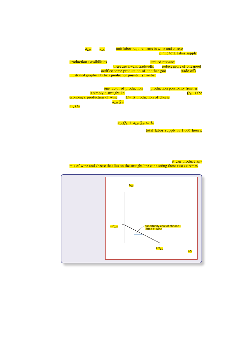
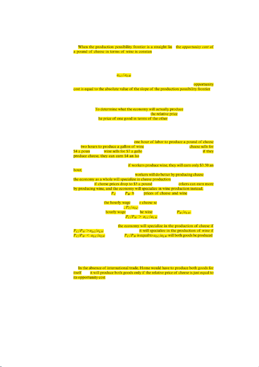
(line PF in Figure 3-1), which
shows the maximum amount of wine that can be produced once the decision has been
made to produce any given amount of cheese, and vice versa. When there is only , the of an economy
e. We can derive this line as follows: If and , then the labor used in producing wine will be
, and the labor used in producing cheese will be
. The production possibility frontier is determined by the limits on the economy’s
resources—in this case, labor. Because the economy’s total labor supply is L, the limits
on production are defined by the inequality (3-1)
Suppose, for example, that the economy’s
and that it takes 1 hour of labor to produce a pound of cheese and 2 hours of
labor to produce a gallon of wine. Then the total labor used in production is
(1 * pounds of cheese produced) + (2 * gallons of wine produced), and this total
must be no more than the 1,000 hours of labor available. If the economy devoted all
its labor to cheese production, it could, as shown in Figure 3-1, produce L>aLC pounds
of cheese (1,000 pounds). If it devoted all its labor to wine production instead, it could
produce L>aLW gallons—1,000>2 = 500 gallons—of wine. And FIGURE 3-1 Home’s Production Home wine production, , Possibility Frontier in gallons The line PF shows the maximum amount of cheese Home can produce given any production of wine, and vice versa.
Absolute value of slope equals P n (500 t gallons in our example) F Home cheese (1,000 pounds production, , in our example) in pounds 56
PART ONE■International Trade Theory e,
t. As we saw in the previous section,
this opportunity cost is defined as the number of gallons of wine the economy would
have to give up in order to produce an extra pound of cheese. In this case, to produce
another pound would require aLC person-hours. Each of these person-hours could in
turn have been used to produce 1>aLW gallons of wine. Thus, the opportunity cost of cheese in terms of wine is
. For example, if it takes one person-hour to make
a pound of cheese and two hours to produce a gallon of wine, the opportunity cost of
each pound of cheese is half a gallon of wine. As Figure 3-1 shows, this . Relative Prices and Supply
The production possibility frontier illustrates the different mixes of goods the economy can produce. , however, we need
to look at prices. Specifically, we need to know of the economy’s two goods, that is, t .
In a competitive economy, supply decisions are determined by the attempts of indi-
viduals to maximize their earnings. In our simplified economy, since labor is the only
factor of production, the supply of cheese and wine will be determined by the move-
ment of labor to whichever sector pays the higher wage.
Suppose, once again, that it takes and . Now suppose further that d, while
n. What will workers produce? Well,
ur. (Bear in mind that since labor is the only
input into production here, there are no profits, so workers receive the full value of
their output.) On the other hand,
because a $7 gallon of wine takes two hours to produce. So if cheese sells for $4 a
pound while wine sells for $7 a gallon, —and . But what ? In that case, w More generally, let and e the , respectively. It
takes aLC person-hours to produce a pound of cheese; since there are no profits in our one-factor model, in th
ctor will equal the value of what a worker can produce in an hour
. Since it takes aLW person-hours to produce a gallon of wine, the rate in t sector will be Wages in the
cheese sector will be higher if
; wages in the wine sector will be
higher if PC>P a a W 6
LC > LW. Because everyone will want to work in whichever indus- try offers the higher wage, . On the other hand, . Only when .
What is the significance of the number a a
LC > LW? We saw in the previous section that
it is the opportunity cost of cheese in terms of wine. We have therefore just derived a
crucial proposition about the relationship between prices and production: The economy
will specialize in the production of cheese if the relative price of cheese exceeds its oppor-
tunity cost in terms of wine; it will specialize in the production of wine if the relative price
of cheese is less than its opportunity cost in terms of wine. . But
. Since opportunity cost equals the ratio of unit labor requirements
CHAPTER 3■Labor Productivity and Comparative Advantage: TheRicardian Model 57
in cheese and wine, we can summarize the determination of prices in the absence of
international trade with a simple labor theory of value: , the r
Trade in a One-Factor World
To describe the pattern and effects of trade between two countries when each country
has only one factor of production is simple. Yet the implications of this analysis can
be surprising. Indeed, to those who have not thought about international trade, many
of these implications seem to conflict with common sense. Even this simplest of trade
models can offer some important guidance on real-world issues, such as what consti-
tutes fair international competition and fair international exchange.
Before we get to these issues, however, let us get the model stated. Suppose there are
two countries. One of them we again call Home and the other we call Foreign. Each
of these countries has one factor of production (labor) and can produce two goods,
wine and cheese. As before, we denote and production by , respectively. For Foreign,
we will use a convenient notation throughout this text: When we refer to some aspect
of Foreign, we will use the same symbol that we use for Home, but with an asterisk. Thus
, Foreign’s unit labor requirements in
wine and cheese will be denoted by
C, respectively, and so on.
In general, the unit labor requirements can follow any pattern. For example,
could be less productive than Foreign in wine but , or vice versa. For the moment, : that (3-2) or, equivalently, that a a LC > L *C 6 a a*
LW> LW. (3-3)
In words, we are assuming that the ratio of the labor required to produce a pound
of cheese to that required to produce a gallon of wine is lower in Home than it is in
Foreign. More briefly still, we are saying that is
But remember that the ratio of unit labor requirements is equal to the opportunity
cost of cheese in terms of wine; and remember also that we defined comparative advan-
tage precisely in terms of such opportunity costs. So the assumption about relative
productivities embodied in equations (3-2) and (3-3) amounts to saying that .
One point should be noted immediately: The condition under which Home has this
comparative advantage involves all four unit labor requirements, not just two. You
might think that to determine who will produce cheese, all you need to do is com-
pare the two countries’ unit labor requirements in cheese production, a * LC and aLC. If
, Home labor is more efficient than Foreign in producing cheese. When one
country can produce a unit of a good with less labor than another country, we say that the first country has an
in producing that good. In our example,
What we will see in a moment, however, is that we cannot determine the pattern of
trade from absolute advantage alone. One of the most important sources of error in dis-
cussing international trade is to confuse comparative advantage with absolute advantage. 58
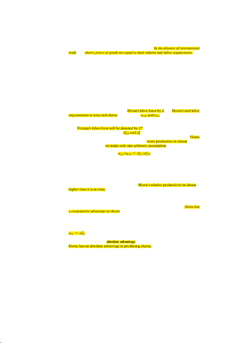
PART ONE■International Trade Theory FIGURE 3-2 Foreign’s Production Foreign wine production, Q , Possibility Frontier W* in gallons
Because Foreign’s relative unit
labor requirement in cheese is
higher than Home’s (it needs to give up many more units of wine to produce one more L*/a* F* LW
unit of cheese), its production
possibility frontier is steeper. P* L*/a* Foreign cheese LC production, Q , C* in pounds
Given the labor forces and the unit labor requirements in the two countries, we can
draw the production possibility frontier for each country. We have already done this
for Home, by drawing PF in Figure 3-1. The production possibility frontier for Foreign
is shown as P*F* in Figure 3-2. Since the slope of the production possibility frontier
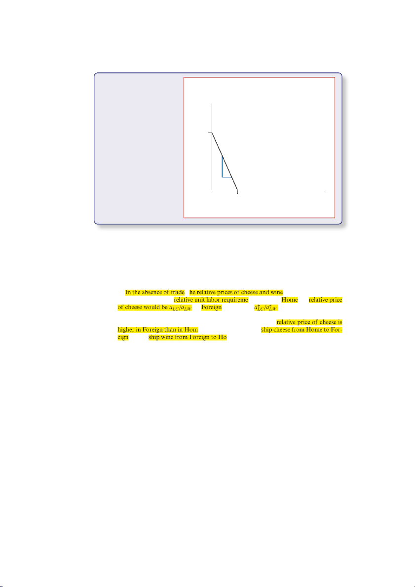
equals the opportunity cost of cheese in terms of wine, Foreign’s frontier is steeper than Home’s. , t in each country would be determined by the nts. Thus, in the ; in it would be
Once we allow for the possibility of international trade, however, prices will no lon-
ger be determined purely by domestic considerations. If the e, it will be profitable to and to
me. This cannot go on indefinitely, however.
Eventually, Home will export enough cheese and Foreign enough wine to equalize the
relative price. But what determines the level at which that price settles?
Determining the Relative Price after Trade
Prices of internationally traded goods, like other prices, are determined by supply and
demand. In discussing comparative advantage, however, we must apply supply-and-
demand analysis carefully. In some contexts, such as some of the trade policy analysis
in Chapters 9 through 12, it is acceptable to focus only on supply and demand in a
single market. In assessing the effects of U.S. import quotas on sugar, for example, it is
reasonable to use partial equilibrium analysis, that is, to study a single market, the sugar
market. When we study comparative advantage, however, it is crucial to keep track of
the relationships between markets (in our example, the markets for wine and cheese).
Since Home exports cheese only in return for imports of wine, and Foreign exports
wine in return for cheese, it can be misleading to look at the cheese and wine markets
CHAPTER 3■Labor Productivity and Comparative Advantage: TheRicardian Model 59
in isolation. What is needed is which
One useful way to keep track of two markets at once is to focus not just on the
quantities of cheese and wine supplied and demanded but also on the relative supply
and demand, that is, on the number of pounds of cheese supplied or demanded divided
by the number of gallons of wine supplied or demanded.
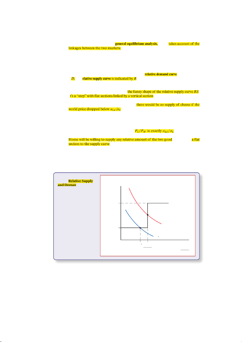
Figure 3-3 shows world supply and demand for cheese relative to wine as functions
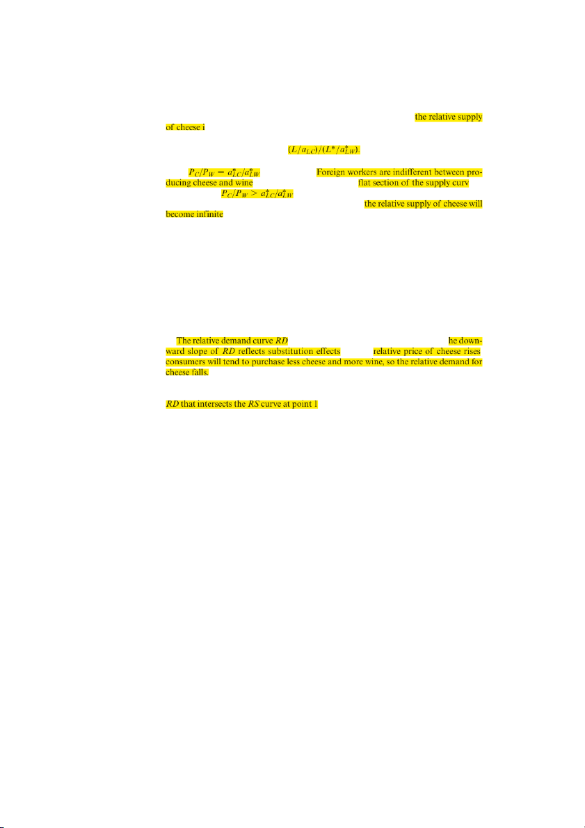
of the price of cheese relative to that of wine. The is indicated by R the r
S. World general equilibrium requires that
relative supply equal relative demand, and thus the world relative price is determined
by the intersection of RD and RS.
The striking feature of Figure 3-3 is : I . Once we understand the deri-
vation of the RS curve, we will be almost home-free in understanding the whole model.
First, as drawn, the RS curve shows that
W. To see why, recall that we showed that Home will
specialize in the production of wine whenever P P
C > W 6 aLC >aLW. Similarly, Foreign
will specialize in wine production whenever P P
C > W 6 aLC
* >a*LW. At the start of our
discussion of equation (3-2), we made the assumption that a a a LC > LW 6 LC
* >a*LW. So at
relative prices of cheese below a a
LC > LW , there would be no world cheese production.
Next, when the relative price of cheese W, we know that
workers in Home can earn exactly the same amount making either cheese or wine. So s, producing .
We have already seen that if P P
C > W is above a a
LC > LW, Home will specialize in the
production of cheese. As long as P P
C > W 6 aLC
* >a*LW, however, Foreign will continue to
specialize in producing wine. When Home specializes in cheese production, it produces FIGURE 3-3 World Relative price of cheese, P /P d C W
The RD and RD’ curves show that the demand for cheese relative to wine is a decreasing function of the aLC * /aLW * RS price of cheese relative to (2 in our
that of wine, while the RS example) curve shows that the supply 1 of cheese relative to wine is an increasing function of the same relative price. RD a 2 LC /aLW (1/2 in our example) RD Q L /a Relative quantity LC L*/a* Q * C + QC LW of cheese, Q * W +QW 60
PART ONE■International Trade Theory L>a *
LC pounds. Similarly, when Foreign specializes in wine, it produces L* > aLW gallons.
So for any relative price of cheese between a a * >a* ,
LC > LW and aLC LW s (3-4) At , we know that . Thus, here we again have a e. Finally, for
, both Home and Foreign will specialize in cheese
production. There will be no wine production, so that .
A numerical example may help at this point. Let’s assume, as we did before, that in
Home it takes one hour of labor to produce a pound of cheese and two hours to pro-
duce a gallon of wine. Meanwhile, let’s assume that in Foreign it takes six hours to pro-
duce a pound of cheese—Foreign workers are much less productive than Home workers
when it comes to cheesemaking—but only three hours to produce a gallon of wine.
In this case, the opportunity cost of cheese production in terms of wine is 1 2 in
Home—that is, the labor used to produce a pound of cheese could have produced half
a gallon of wine. So the lower flat section of RS corresponds to a relative price of 1 2.
Meanwhile, in Foreign the opportunity cost of cheese in terms of wine is 2: The six
hours of labor required to produce a pound of cheese could have produced two gallons
of wine. So the upper flat section of RS corresponds to a relative price of 2.
does not require such exhaustive analysis. T . As the ,
The equilibrium relative price of cheese is determined by the intersection of the
relative supply and relative demand curves. Figure 3-3 shows a relative demand curve
, where the relative price of cheese is between
the two countries’ pretrade prices—say, at a relative price of 1, in between the pretrade
prices of 1 2 and 2. In this case, each country specializes in the production of the good
in which it has a comparative advantage: Home produces only cheese, while Foreign produces only wine.
This is not, however, the only possible outcome. If the relevant RD curve were RD′,
for example, relative supply and relative demand would intersect on one of the horizon-
tal sections of RS. At point 2, the world relative price of cheese after trade is a a LC > LW,
the same as the opportunity cost of cheese in terms of wine in Home.
What is the significance of this outcome? If the relative price of cheese is equal to
its opportunity cost in Home, the Home economy need not specialize in producing
either cheese or wine. In fact, at point 2 Home must be producing both some wine and
some cheese; we can infer this from the fact that the relative supply of cheese (point
Q′ on the horizontal axis) is less than it would be if Home were in fact completely specialized. Since P P
C > W is below the opportunity cost of cheese in terms of wine in
Foreign, however, Foreign does specialize completely in producing wine. It therefore
remains true that if a country does specialize, it will do so in the good in which it has a comparative advantage.
For the moment, let’s leave aside the possibility that one of the two countries does
not completely specialize. Except in this case, the normal result of trade is that the
price of a traded good (e.g., cheese) relative to that of another good (wine) ends up
somewhere in between its pretrade levels in the two countries. 62
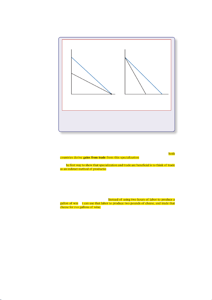
PART ONE■International Trade Theory Quantity Quantity of wine, QW of wine, QW* T F* P F P* T* Quantity Quantity of cheese, QC of cheese, QC * (a) Home (b) Foreign FIGURE 3-4
Trade Expands Consumption Possibilities
International trade allows Home and Foreign to consume anywhere within the colored lines,
which lie outside the countries’ production frontiers. The Gains from Trade
We have now seen that countries whose relative labor productivities differ across
industries will specialize in the production of different goods. We next show that . This mutual gain can be
demonstrated in two alternative ways. T
n. Home could produce wine directly, but trade with
Foreign allows it to “produce” wine by producing cheese and then trading the cheese for
wine. This indirect method of “producing” a gallon of wine is a more efficient method than direct production.
Consider our numerical example yet again: In Home, we assume that it takes one
hour to produce a pound of cheese and two hours to produce a gallon of wine. This
means that the opportunity cost of cheese in terms of wine is 1 2. But we know that the
relative price of cheese after trade will be higher than this, say 1. So here’s one way to
see the gains from trade for Home: e, i
More generally, consider two alternative ways of using an hour of labor. On one
side, Home could use the hour directly to produce 1>aLW gallons of wine. Alternatively,
Home could use the hour to produce 1>aLC pounds of cheese. This cheese could then
be traded for wine, with each pound trading for P P
C > W gallons, so our original hour
CHAPTER 3■Labor Productivity and Comparative Advantage: TheRicardian Model 63 of labor yields (1>a )( LC
PC>PW) gallons of wine. (3-5) or .
But we just saw that in international equilibrium, if neither country produces both goods,
. This shows that Home can “produce” wine
more efficiently by making cheese and trading it than by producing wine directly for
itself. Similarly, Foreign can “produce” cheese more efficiently by making wine and
trading it. This is one way of seeing that both countries gain.
Another way to see the mutual gains from trade is to examine how trade affects each
country’s possibilities for consumption. In the absence of trade, consumption possibili-
ties are the same as production possibilities (the solid lines PF and P*F* in Figure 3-4).
Once trade is allowed, however, each economy can consume a different mix of cheese
and wine from the mix it produces. Home’s consumption possibilities are indicated
by the colored line TF in Figure 3-4a, while Foreign’s consumption possibilities are
indicated by T*F* in Figure 3-4b. In each case, trade has enlarged the range of choice,
and therefore it must make residents of each country better off. A Note on Relative Wages
Political discussions of international trade often focus on comparisons of wage rates
in different countries. For example, opponents of trade between the United States
and Mexico often emphasize the point that workers in Mexico are paid only about
$6.50 per hour, compared with more than $35 per hour for the typical worker in the
United States. Our discussion of international trade up to this point has not explicitly
compared wages in the two countries, but it is possible in the context of our numerical
example to determine how the wage rates in the two countries compare.
In our example, once the countries have specialized, all Home workers are employed
producing cheese. Since it takes one hour of labor to produce one pound of cheese,
workers in Home earn the value of one pound of cheese per hour of their labor. Simi-
larly, Foreign workers produce only wine; since it takes three hours for them to produce
each gallon, they earn the value of 1 3 of a gallon of wine per hour.
To convert these numbers into dollar figures, we need to know the prices of cheese
and wine. Suppose that a pound of cheese and a gallon of wine both sell for $12; then
Home workers will earn $12 per hour, while Foreign workers will earn $4 per hour. The
relative wage of a country’s workers is the amount they are paid per hour, compared
with the amount workers in another country are paid per hour. The relative wage of
Home workers will therefore be 3.
Clearly, this relative wage does not depend on whether the price of a pound of
cheese is $12 or $20, as long as a gallon of wine sells for the same price. As long as
the relative price of cheese—the price of a pound of cheese divided by the price of a
gallon of wine—is 1, the wage of Home workers will be three times that of Foreign workers.
Notice that this wage rate lies between the ratios of the two countries’ productivities
in the two industries. Home is six times as productive as Foreign in cheese, but only
one-and-a-half times as productive in wine, and it ends up with a wage rate three times
CHAPTER 3■Labor Productivity and Comparative Advantage: TheRicardian Model 73
Even at a relative Home wage of 3, which makes this the equivalent of 9 hours of For-
eign labor, this is cheaper than the 12 hours Foreign would need to produce caviar for
itself. In the absence of transport costs, then, Foreign would find it cheaper to import
caviar than to make it domestically. With a 100 percent cost of transportation, however,
imported caviar would cost the equivalent of 18 hours of Foreign labor and would
therefore be produced locally instead.
The result of introducing transport costs in this example, then, is that Home will still
export apples and bananas and import enchiladas, but caviar and dates will become
nontraded goods, which each country will produce for itself.
In this example, we have assumed that transport costs are the same fraction of
production cost in all sectors. In practice there is a wide range of transportation
costs. In some cases transportation is virtually impossible: Services such as haircuts
and auto repair cannot be traded internationally (except where there is a metropoli-
tan area that straddles a border, like Detroit, Michigan–Windsor, Ontario). There is
also little international trade in goods with high weight-to-value ratios, like cement.
(It is simply not worth the transport cost of importing cement, even if it can be
produced much more cheaply abroad.) Many goods end up being nontraded either
because of the absence of strong national cost advantages or because of high trans- portation costs.
The important point is that nations spend a large share of their income on non-
traded goods. This observation is of surprising importance in our later discussion of
international monetary economics.
Empirical Evidence on the Ricardian Model
The Ricardian model of international trade is an extremely useful tool for thinking
about the reasons why trade may happen and about the effects of international trade
on national welfare. But is the model a good fit to the real world? Does the Ricardian
model make accurate predictions about actual international trade flows?
The answer is a heavily qualified yes. Clearly
. First, as mentioned in our discus-
sion of nontraded goods, the simple Ricardian model predicts an extreme degree of
specialization that we do not observe in the real world. Second, t
and thus predicts that countries as a whole will always gain from trade; in practice, i . Third, the Ricardian model allows m (the focus of
Chapters 4 and 5). Finally, the Ricardian model , which leaves it unable to
—an issue discussed in Chapters 7 and 8.
In spite of these failings, however, the basic prediction of the Ricardian model—that
has been strongly confirmed by a number of studies over the years.
Several classic tests of the Ricardian model, performed using data from the early
post-World War II period, compared British with American productivity and trade.4
4The pioneering study by G. D. A. MacDougall is listed in Further Readings at the end of the chapter.
Awell-known follow-up study, on which we draw here, was Bela Balassa, “An Empirical Demonstration of
Classical Comparative Cost Theory,” Review of Economics and Statistics 45 (August 1963), pp. 231–238; we
use Balassa’s numbers as an illustration.
CHAPTER 3■Labor Productivity and Comparative Advantage: TheRicardian Model 75
products; the relative productivity must be high compared with relative productivity
in other sectors. As it happened, U.S. productivity exceeded British productivity in
all 26sectors (indicated by dots) shown in Figure 3-6, by margins ranging from 11 to
366 percent. In 12 of the sectors, however, Britain actually had larger exports than the
United States. A glance at the figure shows that, in general, U.S. exports were larger than
U.K. exports only in industries where the U.S. productivity advantage was somewhat more than two to one.
More recent evidence on the Ricardian model has been less clear-cut. In part, this is
because the growth of world trade and the resulting specialization of national econo-
mies means that we do not get a chance to see what countries do badly! In the world economy of ry, , so th . For example,
id. Nonetheless, several pieces of
evidence suggest that differences in labor productivity continue to play an important
role in determining world trade patterns. Perhaps s of the
Ricardian theory of comparative advantage is the wa
Consider, for example, the case of clothing exports from Bangladesh. The
Bangladeshi clothing industry received the worst kind of publicity in April 2013,
when a building housing five garment factories collapsed, killing more than a thou-
sand people. The backstory to this tragedy, however, was the growth of Bangla-
desh’s clothing exports, which were rapidly gaining on those of China, previously
the dominant supplier. This rapid growth took place even though Bangladesh is
a very, very poor country, with extremely low overall productivity even compared
with China, which as we have already seen is still low-productivity compared with the United States.
What was the secret of Bangladesh’s success? —but
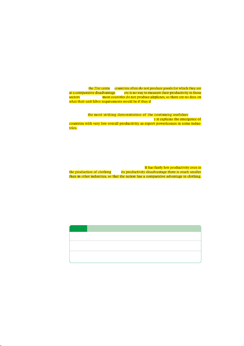
Table 3-3 illustrates this point with some estimates based on 2011 data.
Compared with China, Bangladesh still has an absolute disadvantage in clothing
production, with significantly lower productivity. But because its relative productivity
in apparel is so much higher than in other industries, Bangladesh has a strong com-
parative advantage in apparel—and its apparel industry is giving China a run for the money.
In sum, while few economists believe that the Ricardian model is a fully ade-
quate description of the causes and consequences of world trade, its two principal
TABLE 3-3 Bangladesh versus China, 2011
Bangladeshi Output per Worker Bangladeshi Exports as % of China as % of China All industries 28.5 1.0 Apparel 77 15.5
Source: McKinsey and Company, “Bangladesh’s ready-made garments industry: The challenge of
growth,” 2012; UN Monthly Bulletin of Statistics.