Lecture 3 - ENEE1006IU

lOMoARcPSD|359 747 69 APPLIED STATISTICS COURSE CODE: ENEE1006IU Lecture 3:
Chapter 2: Plotting and Smoothing data
(3 credits: 2 is for lecture, 1 is for lab-work)
Instructor: TRAN THANH TU Email: tttu@hcmiu.edu.vn tttu@hcmiu.edu.vn 1 lOMoARcPSD|359 747 69 2.1. PLOTTING DATA
•The first step in data analysis should be to plot the data. Graphing data should be
an interactive experimental process.
•Make a variety of graphs to view the data in different ways. Doing this may:
1. Reveal the answer so clearly that little more analysis is needed
2. Point out properties of the data that would invalidate a particular statisticalanalysis
3. Reveal that the sample contains unusual observations
4. Save time in subsequent analyses
5. Suggest an answer that you had not expected6. Keep you from doing something foolish tttu@hcmiu.edu.vn lOMoARcPSD|359 747 69 tttu@hcmiu.edu.vn 2 2.1. PLOTTING DATA
Number (frequency) The relative frequency of observations 100 frequency of a class is
in Divided by n of a class equals the the relative frequency
each of several non- fraction or proportion overlapping multiplied by 100.
of observations categories or classes. belonging to a class.
A frequency distribution is a tabular summary of A A percent frequency relative frequency distribution data showing the number distribution gives a summarizes the
(frequency) of tabular summary of data observations in percent frequency of each of
showing the relative several non-overlapping the data for each class.
frequency for each categories or classes. class. 3 The percent Multiply lOMoARcPSD|359 747 69 2.1. PLOTTING DATA
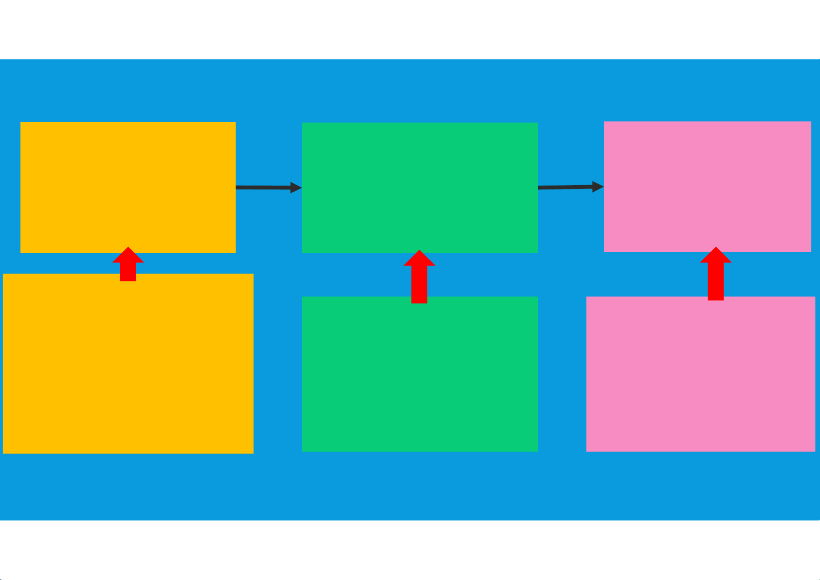
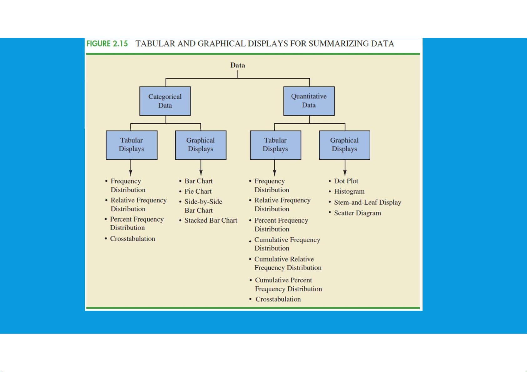
•Displays Used to Show the Distribution of Data:
Bar Chart: show the frequency distribution and relative frequency distribution for categorical data
Pie Chart: show the relative frequency and percent frequency for categorical data
Dot Plot: show the distribution for quantitative data over the entire range of the data
Histogram: show the frequency distribution for quantitative data over a set of class intervals
Stem-and-Leaf display: show both the rank order and shape of the distribution for quantitative data tttu@hcmiu.edu.vn lOMoARcPSD|359 747 69 4 2.1. PLOTTING DATA
•Displays Used to Show the Distribution of Data:
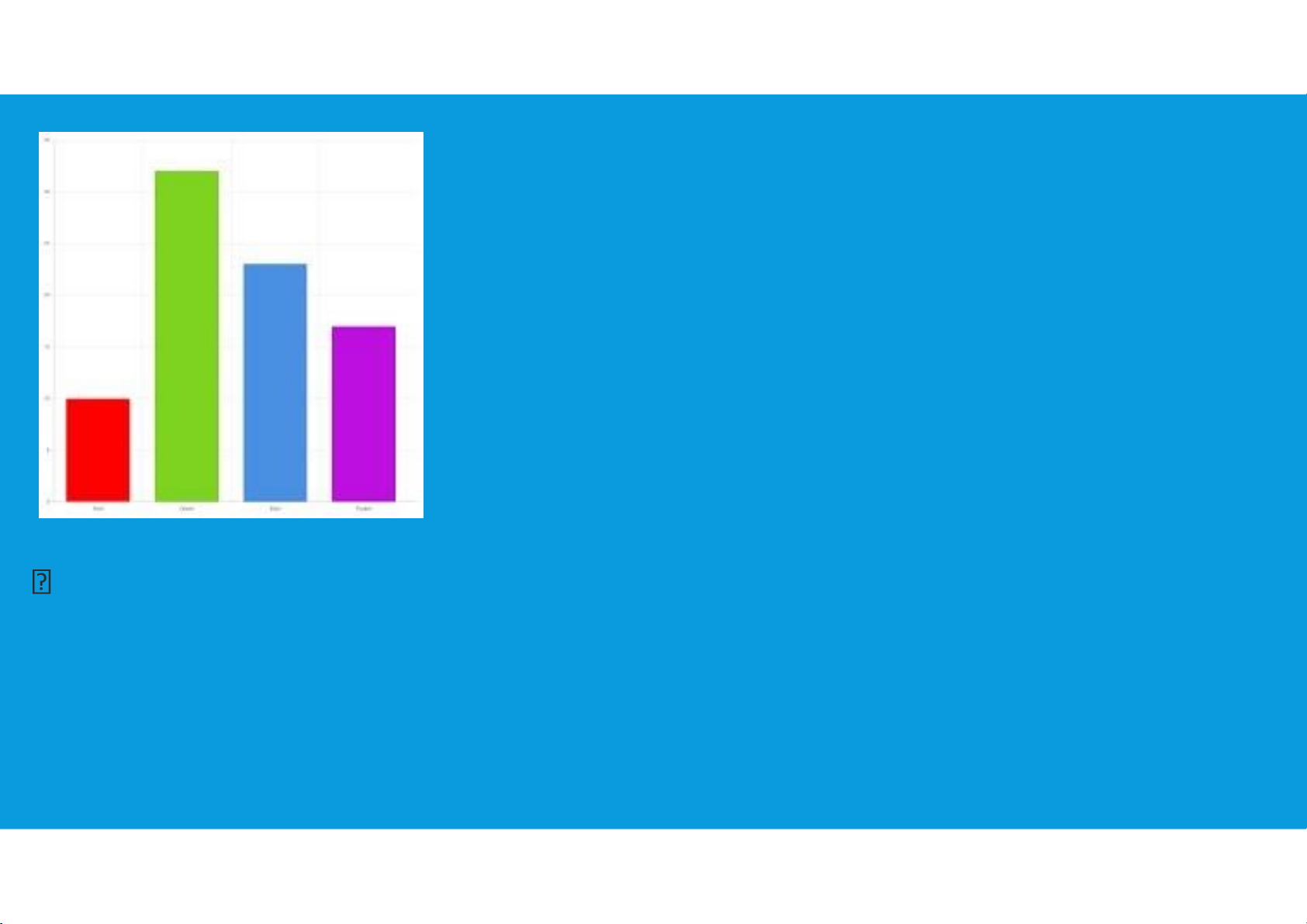
Bar Chart: show the frequency, relative frequency, percent frequency
distributions for categorical data tttu@hcmiu.edu.vn lOMoARcPSD|359 747 69 •
On one axis of the chart (usually the horizontal
axis), we specify the labels that are used for the classes (categories). •
A frequency, relative frequency, or percent
frequency scale can be used for the other axis of
the chart (usually the vertical axis). 5 2.1. PLOTTING DATA
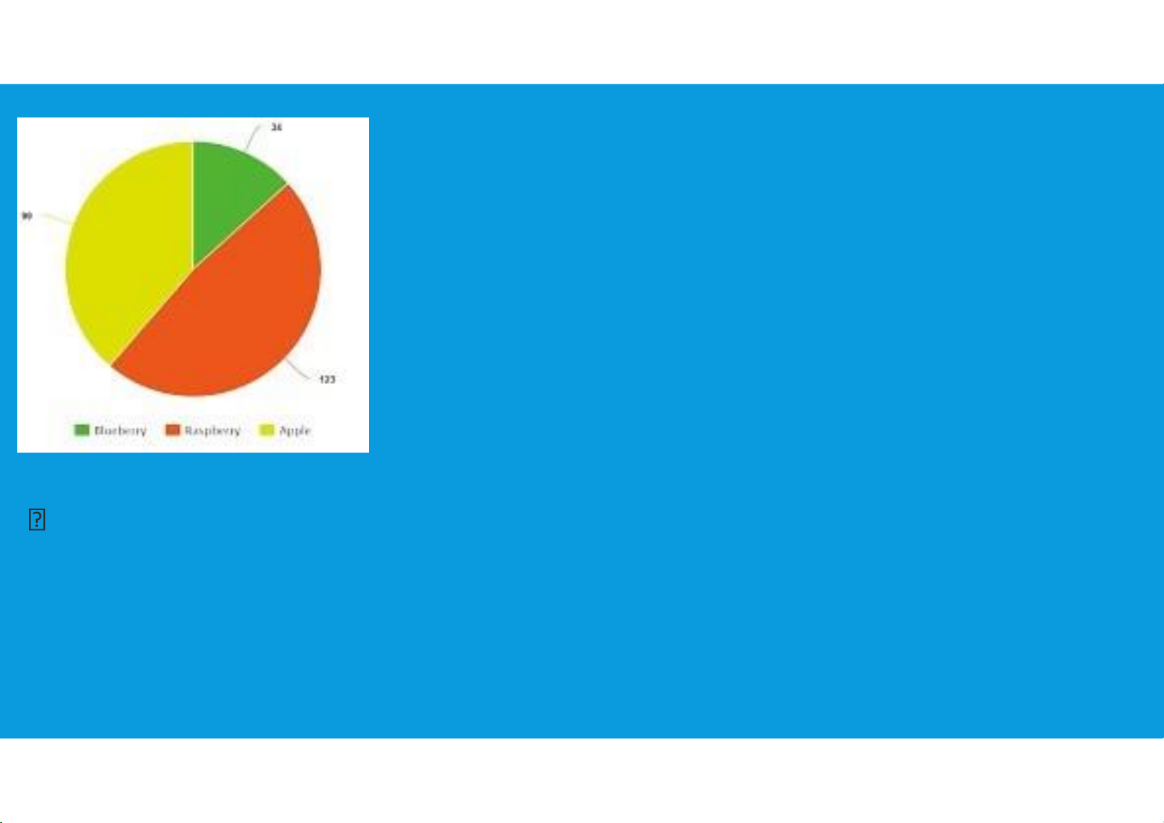
•Displays Used to Show the Distribution of Data:
Pie Chart: show the relative frequency and percent frequency distributions for categorical data tttu@hcmiu.edu.vn lOMoARcPSD|359 747 69
• First, draw a circle to represent all the data.
• Then, use the relative frequencies to subdivide the
circle into sectors, or parts, that correspond to the
relative frequency for each class. 6 2.1. PLOTTING DATA
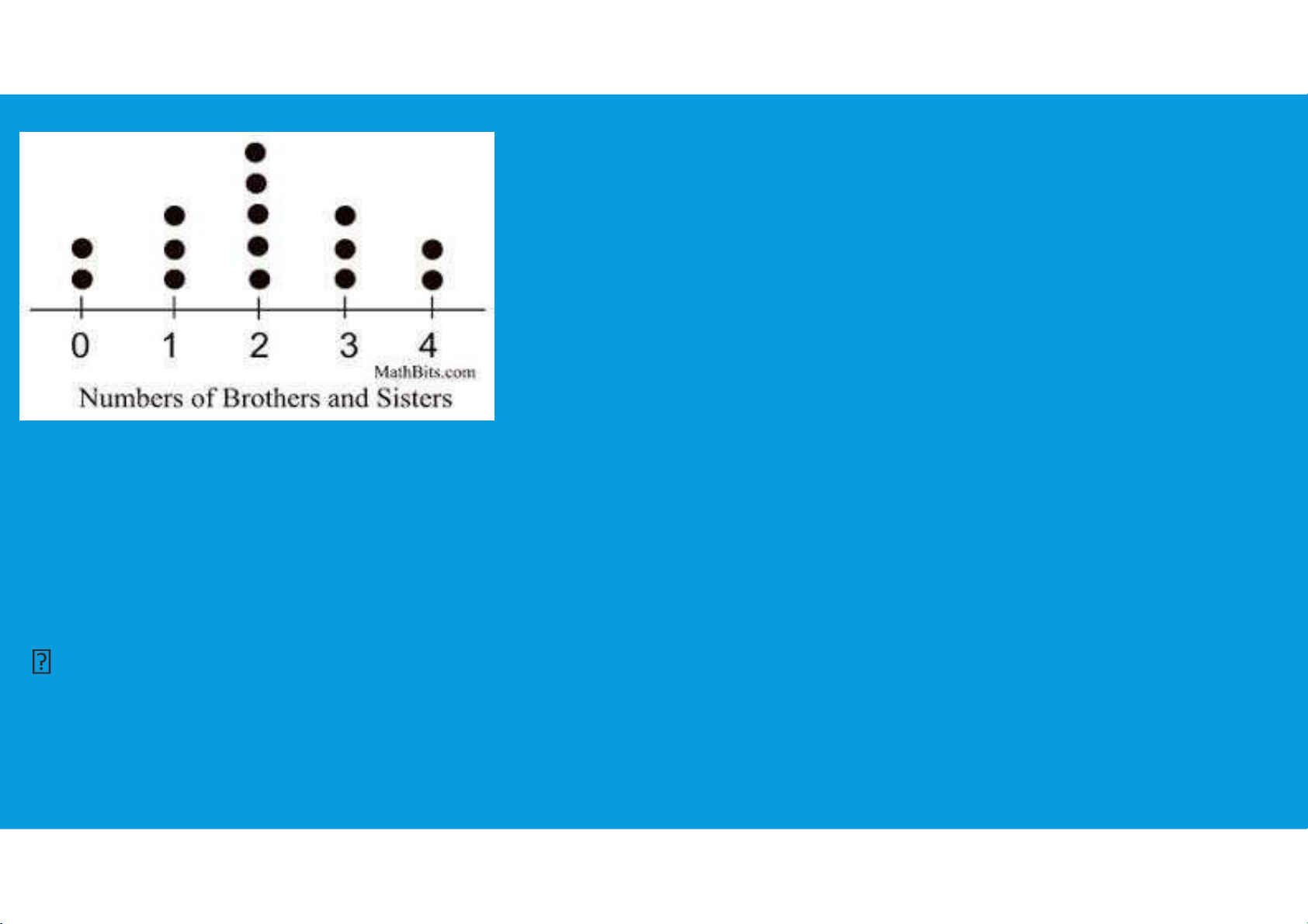
•Displays Used to Show the Distribution of Data:
Dot Plot: show the distribution for quantitative data over the entire range of the data tttu@hcmiu.edu.vn lOMoARcPSD|359 747 69
• A horizontal axis shows the range for the data.
• Each data value is represented by a dot placed above the axis. 7 2.1. PLOTTING DATA
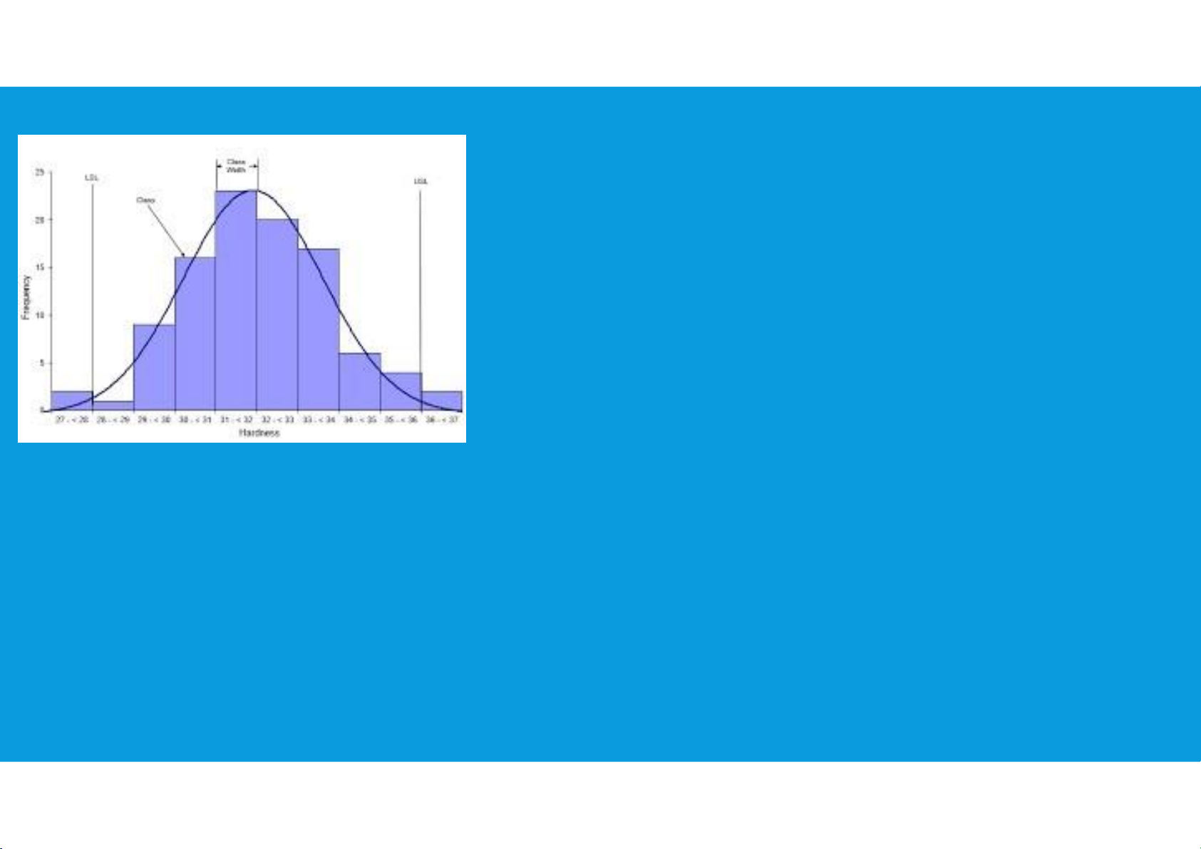
•Displays Used to Show the Distribution of Data:
Histogram: show the frequency distribution for quantitative data over a set of class intervals tttu@hcmiu.edu.vn lOMoARcPSD|359 747 69
• Place the variable of interest on the horizontal axis and the frequency, histogram contains no natural
relative frequency, or percent
separation between the rectangles
frequency on the vertical axis.
• Draw a rectangle whose base is determined by
the class limits on the horizontal axis and whose
height is the corresponding frequency, relative
frequency, or percent frequency. 8 2.1. PLOTTING DATA
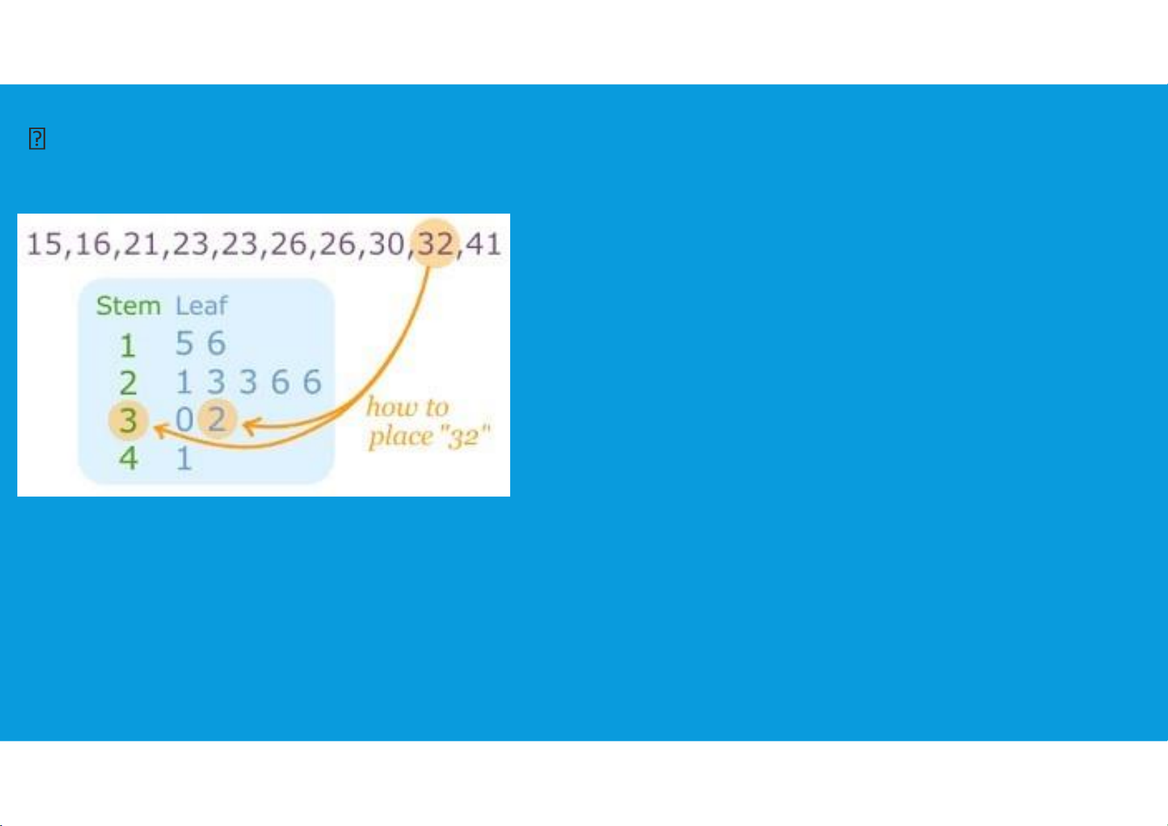
•Displays Used to Show the Distribution of Data: tttu@hcmiu.edu.vn lOMoARcPSD|359 747 69
Stem-and-Leaf display: show both the rank order and shape of the distribution for quantitative data
• The stem-and-leaf display is easier to construct by hand.
• Within a class interval, the stemand-leaf
display provides more information than the
histogram because the stem-and-leaf shows the actual data. 9 tttu@hcmiu.edu.vn lOMoARcPSD|359 747 69 2.1. PLOTTING DATA
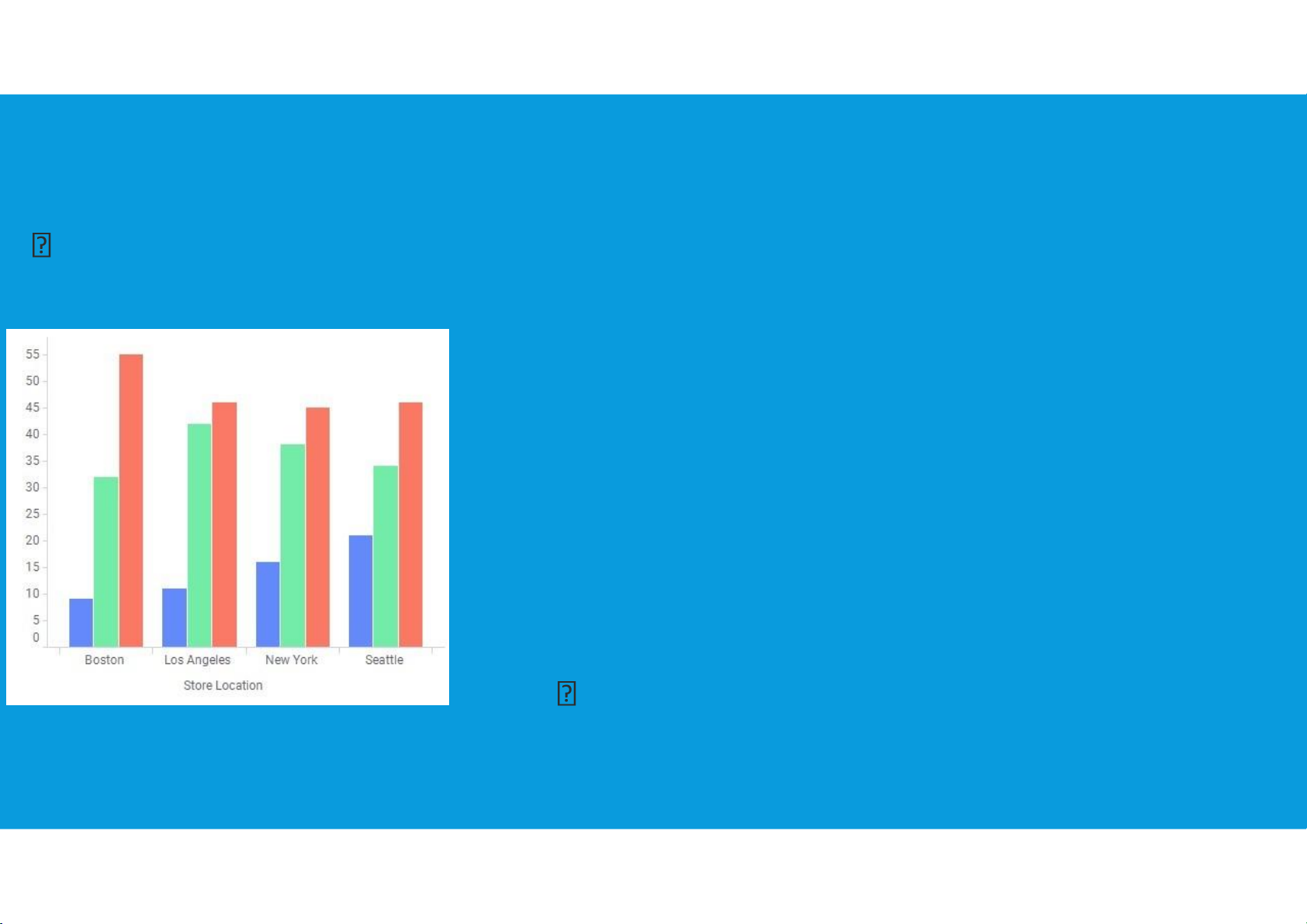
•Displays Used to Make Comparisons:
Side-by-Side bar Chart: a graphical display for depicting multiple bar charts on the same display compare two variables tttu@hcmiu.edu.vn 10 lOMoARcPSD|359 747 69 2.1. PLOTTING DATA
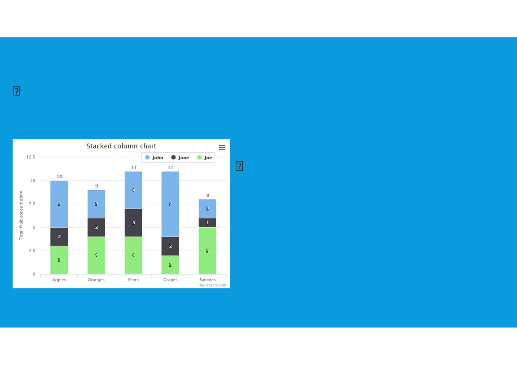
•Displays Used to Make Comparisons:
Stacked bar Charts: a bar chart in which each bar is broken into rectangular
segments of a different color showing the relative frequency of each class in a
manner similar to a pie chart.
compare the relative frequency or percent
frequency of two categorical variables tttu@hcmiu.edu.vn 11 lOMoARcPSD|359 747 69 2.1. PLOTTING DATA
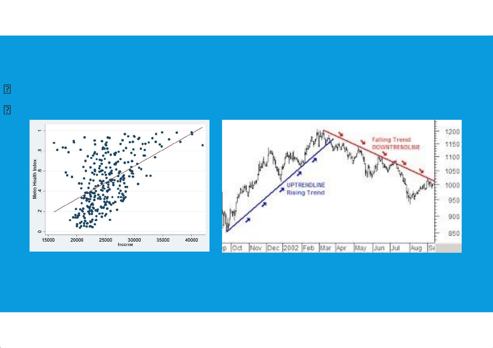
•Displays Used to Show Relationships:
Scatter plot/diagram: show the relationship between two quantitative variables.
Trendline: approximate the relationship of data in a scatter diagram. tttu@hcmiu.edu.vn 12 lOMoARcPSD|359 747 69 2.1. PLOTTING DATA •Scatterplot:
•Simple scatterplots are often made before any other data analysis is considered.
•The insights gained may lead to more elegant and informative graphs, or suggest a promising model.
•Linear or nonlinear relations are easily seen, and so are outliers or other aberrations in the data. tttu@hcmiu.edu.vn 13 lOMoARcPSD|359 747 69 lOMoARcPSD|359 747 69 tttu@hcmiu.edu.vn 14 2.2. SMOOTHING DATA
•Smoothing is drawing a smooth curve through data in order to eliminate the
roughness (scatter) that blurs the fundamental underlying pattern.
•Smoothing can be thought of as a decomposition of the data.
•In smoothing, the analogous expression is: Data = smooth + rough tttu@hcmiu.edu.vn 15 lOMoARcPSD|359 747 69 2.2. SMOOTHING DATA
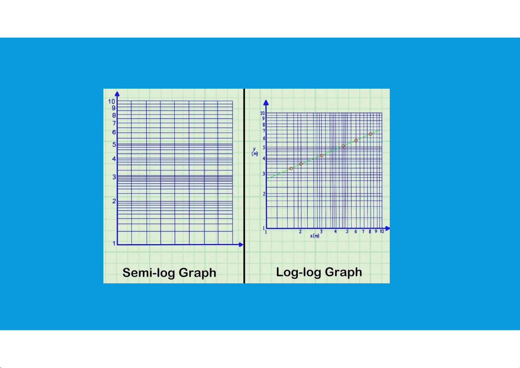
•The simplest smoothing method is to plot the data on a logarithmic scale (or plot
the logarithm of y instead of y itself).
•A logarithmic scale is a nonlinear scale often used when analyzing a large range of quantities.
•Smoothing by plotting the moving averages (MA) or exponentially weighted
moving averages (EWMA) requires only arithmetic (addition, subtraction, multiplication and division).
•The choice of a smoothing method might be influenced by the application. tttu@hcmiu.edu.vn 16 lOMoARcPSD|359 747 69 2.2. SMOOTHING DATA
•Plotting on a Logarithmic Scale: tttu@hcmiu.edu.vn 17 lOMoARcPSD|359 747 69 2.2. SMOOTHING DATA
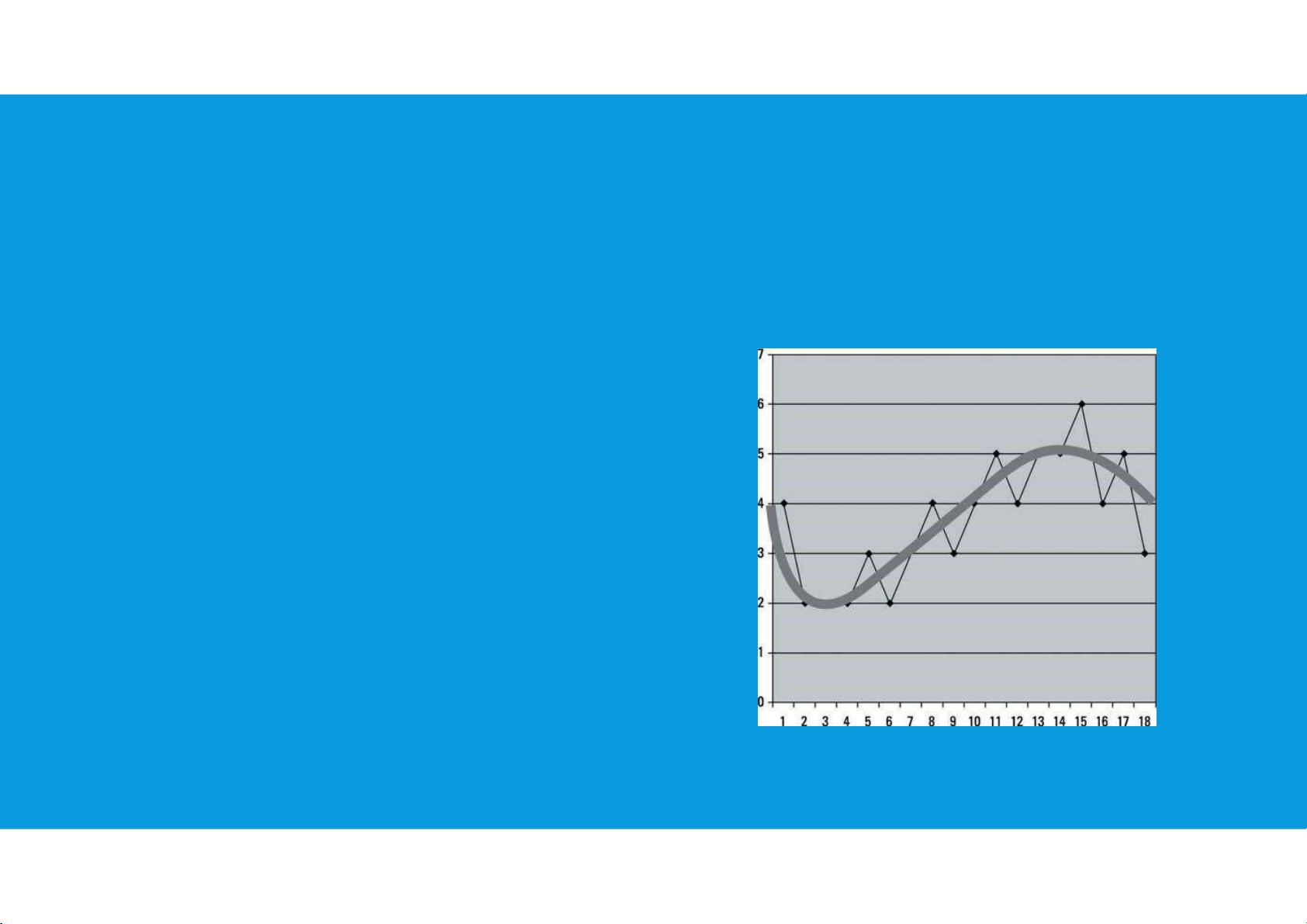
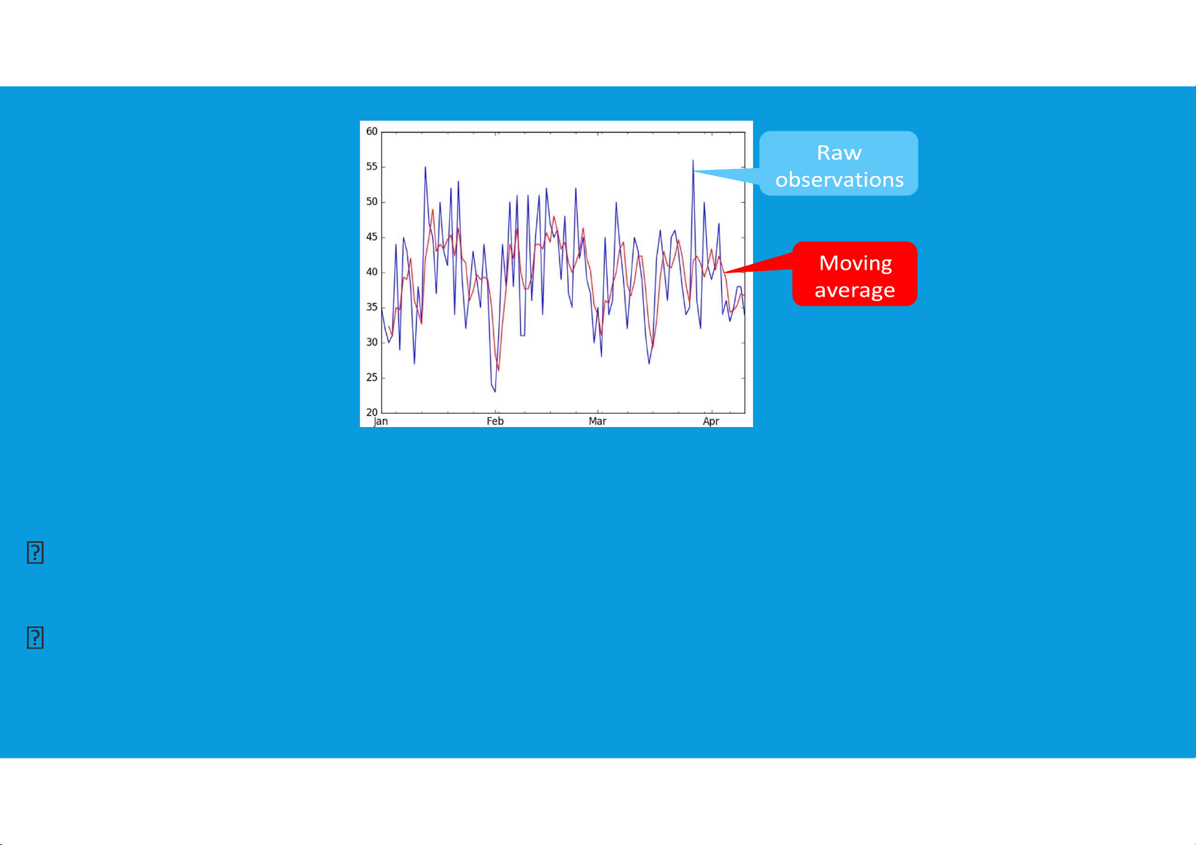
•Smoothing by plotting the moving averages (MA): Moving averages are a simple
and common type of smoothing used in time series analysis and time series forecasting.
Calculating a moving average involves creating a new series where the values
are comprised of the average of raw observations in the original time series. tttu@hcmiu.edu.vn 18 lOMoARcPSD|359 747 69 2.2. SMOOTHING DATA
•Smoothing by plotting the moving averages (MA):
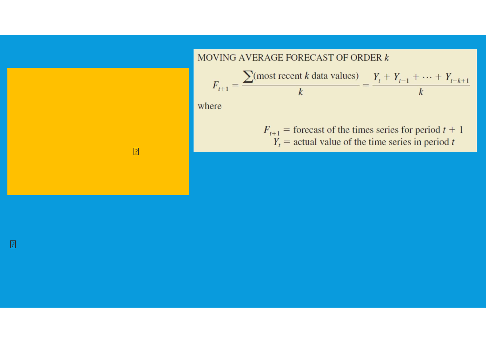
The moving averages method uses the average of the most recent k data values
in the time series as the forecast for the next period.
Mathematically, a moving average forecast of order k is as follows: tttu@hcmiu.edu.vn 19 lOMoARcPSD|359 747 69
The term moving is used because every time a new observation
becomes available for the time
series, it replaces the oldest
observation in the equation and a new average is computed. The
average will change, or move, as new
observations become available. 2.2. SMOOTHING DATA
•Smoothing by plotting the moving averages (MA):
To use moving averages to forecast a time series, we must first select the order, or number of
time series values, to be included in the moving average. tttu@hcmiu.edu.vn 20 lOMoARcPSD|359 747 69
- If only the most recent values of the time series are considered relevant, a small value of k is preferred.
- If more past values are considered relevant, then a larger value of k is better.
As mentioned earlier, a time series with a horizontal pattern can shift to a new level over time.
A moving average will adapt to the new level of the series and resume providing good forecasts in k periods.
Thus, a smaller value of k will track shifts in a time series more quickly.
But larger values of k will be more effective in smoothing out the random fluctuations over time. tttu@hcmiu.edu.vn 21 lOMoARcPSD|359 747 69 2.2. SMOOTHING DATA
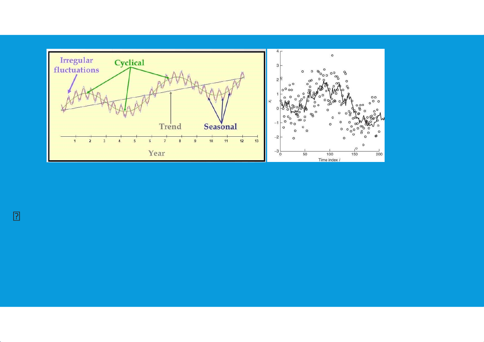
•Smoothing by plotting the exponentially weighted moving averages
(EWMA): The EWMA is often used for smoothing irregular fluctuations (i.e., noise)
in a time series to permit the data analyst to better reveal trend/cycle patterns over time.
•Additionally, the EWMA is frequently used to compute short-term forecasts of
time series (e.g., sales and stocks) lOMoARcPSD|359 747 69 tttu@hcmiu.edu.vn 21 2.2. SMOOTHING DATA
•Smoothing by plotting the exponentially weighted moving averages (EWMA):
Weighted moving averages involves selecting a different weight for each data
value and then computing a weighted average of the most recent k values as the forecast. lOMoARcPSD|359 747 69
In most cases, the most recent observation receives the most weight, and the
weight decreases for older data values. sum of the weights is equal to 1 tttu@hcmiu.edu.vn 22 2.2. SMOOTHING DATA
•Smoothing by plotting the exponentially weighted moving averages (EWMA):
•Forecast accuracy: to use the weighted moving averages method, we must first
select the number of data values to be included in the weighted moving average
and then choose weights for each of the data values. lOMoARcPSD|359 747 69
•In general, if we believe that the recent past is a better predictor of the future
than the distant past, larger weights should be given to the more recent observations.
•However, when the time series is highly variable, selecting approximately equal
weights for the data values may be best. The only requirement in selecting the
weights is that their sum must equal 1. tttu@hcmiu.edu.vn 23
Document Outline

• APPLIED STATISTICS
  • 2.1. PLOTTING DATA
  • 2.1. PLOTTING DATA (1)
  • 2.1. PLOTTING DATA (2)
  • 2.1. PLOTTING DATA (3)
  • 2.1. PLOTTING DATA (4)
  • 2.1. PLOTTING DATA (5)
  • 2.1. PLOTTING DATA (6)
  • 2.1. PLOTTING DATA (7)
  • 2.1. PLOTTING DATA (8)
  • 2.1. PLOTTING DATA (9)
  • 2.1. PLOTTING DATA (10)
  • 2.1. PLOTTING DATA (11)
  • 2.2. SMOOTHING DATA
  • 2.2. SMOOTHING DATA (1)
  • 2.2. SMOOTHING DATA (2)
  • 2.2. SMOOTHING DATA (3)
  • 2.2. SMOOTHING DATA (4)
  • 2.2. SMOOTHING DATA (5)
  • 2.2. SMOOTHING DATA (6)
  • 2.2. SMOOTHING DATA (7)
  • 2.2. SMOOTHING DATA (8)