Lecture 6 - ENEE1006IU

lOMoARcPSD|364 906 32 APPLIED STATISTICS COURSE CODE: ENEE1006IU Lecture 6:
Chapter 4: Probability and Distribution
(3 credits: 2 is for lecture, 1 is for lab-work)
Instructor: TRAN THANH TU Email: tttu@hcmiu.edu.vn tttu@hcmiu.edu.vn 1 lOMoARcPSD|364 906 32
4.1. INTRODUCTION TO PROBABILITY
•Random experiments, counting rules, and assigning probabilities
•Events and their probabilities
•Some basic relationships of probability •Conditional probability •Bayes’ theorem
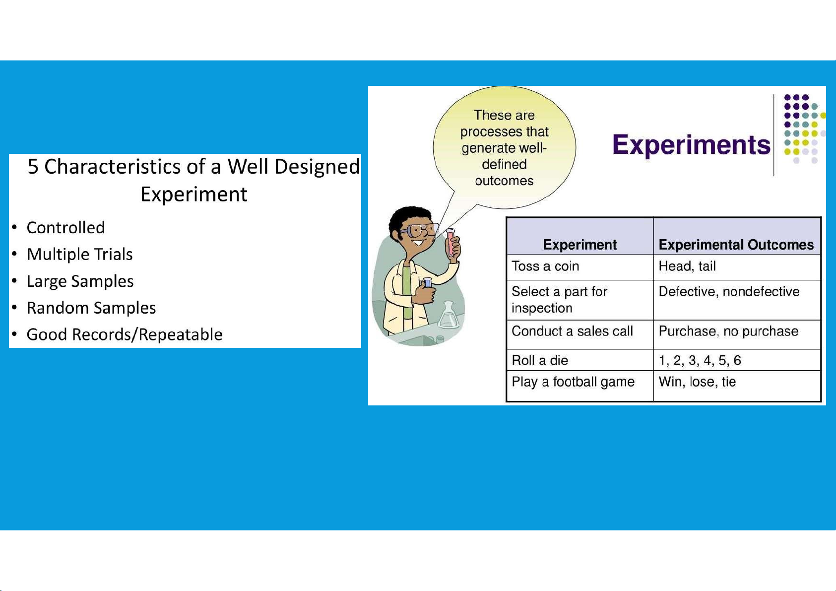
4.1. INTRODUCTION TO PROBABILITY tttu@hcmiu.edu.vn 2 lOMoARcPSD|364 906 32 •Random experiments:
A random experiment is a process that generates well-defined experimental
outcomes. On any single repetition or trial, the outcome that occurs is
determined completely by chance.
By specifying all the possible experimental outcomes, we identify the sample
space for a random experiment.
The sample space for a random experiment is the set of all experimental outcomes.
An experimental outcome is also called a sample point to identify it as an element of the sample space.
4.1. INTRODUCTION TO PROBABILITY •Random experiments: tttu@hcmiu.edu.vn 3 lOMoARcPSD|364 906 32
4.1. INTRODUCTION TO PROBABILITY •Counting rules: tttu@hcmiu.edu.vn 4 lOMoARcPSD|364 906 32
Being able to identify and count the experimental outcomes is a necessary step in assigning probabilities. Three useful counting rules:
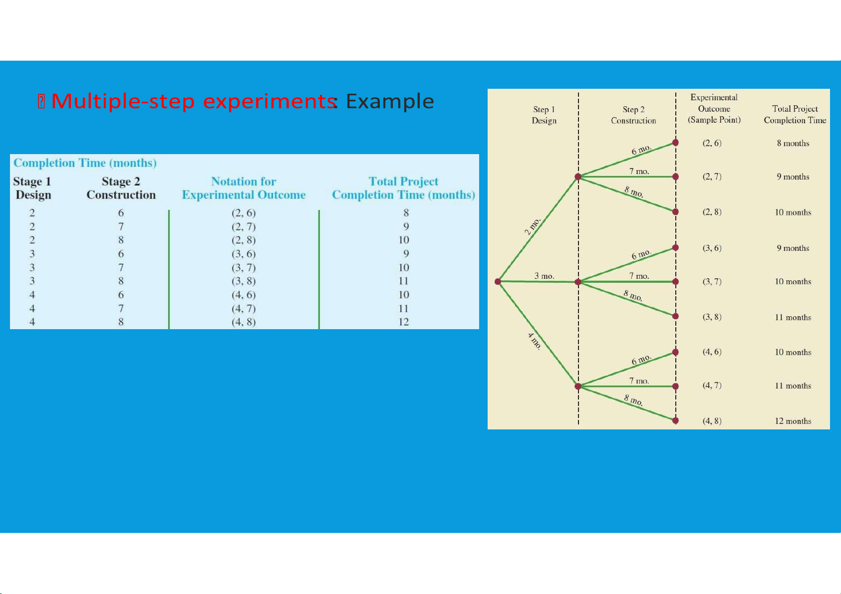
Multiple-step experiments: If an experiment can be described as a sequence of k
steps with n1 possible outcomes on the first step, n2 possible outcomes on the
second step, and so on, then the total number of experimental outcomes is given by (n1)*(n2)* . . . *(nk).
4.1. INTRODUCTION TO PROBABILITY •Counting rules: tttu@hcmiu.edu.vn 5 lOMoARcPSD|364 906 32
4.1. INTRODUCTION TO PROBABILITY tttu@hcmiu.edu.vn 6 lOMoARcPSD|364 906 32 •Counting rules:
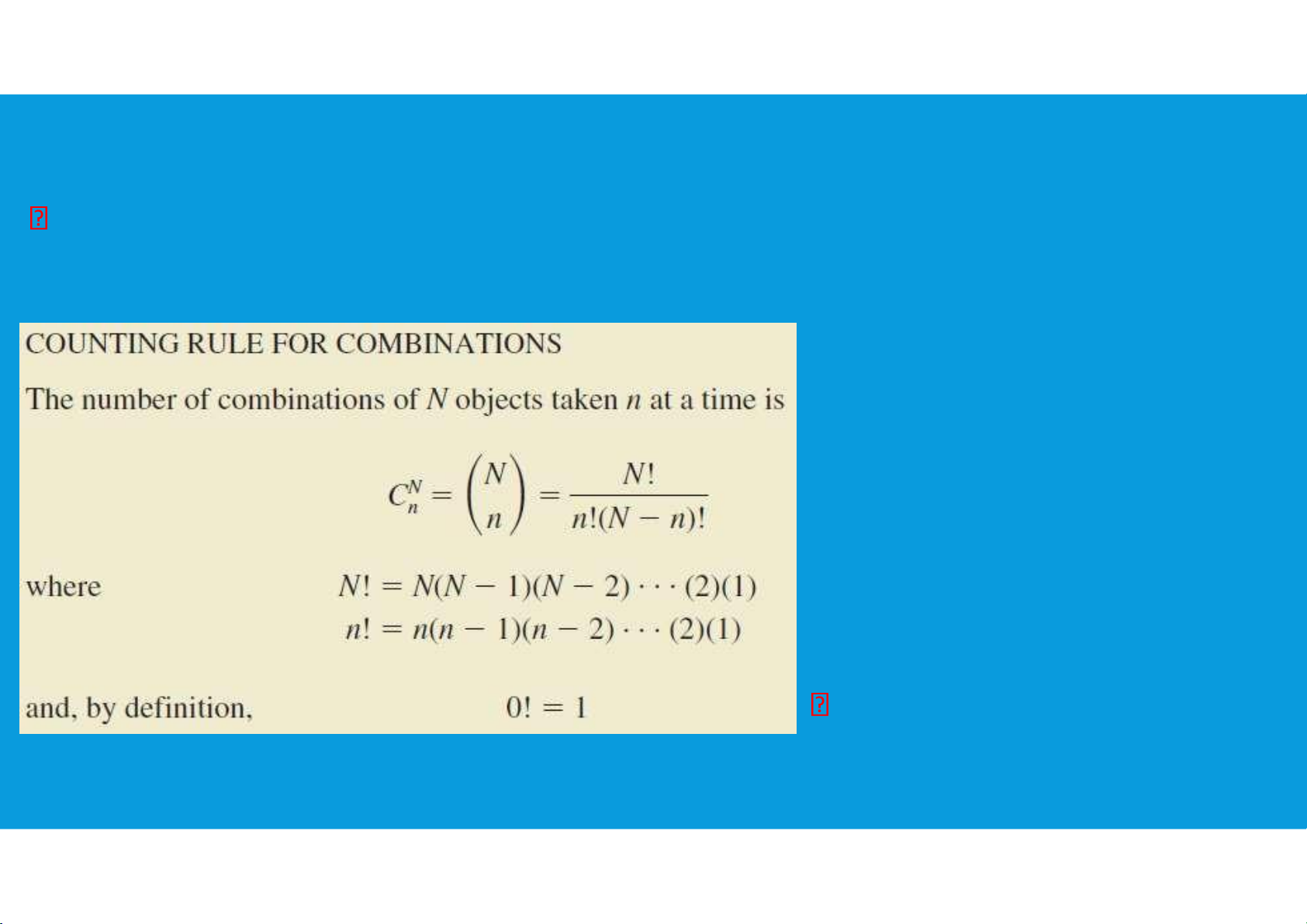
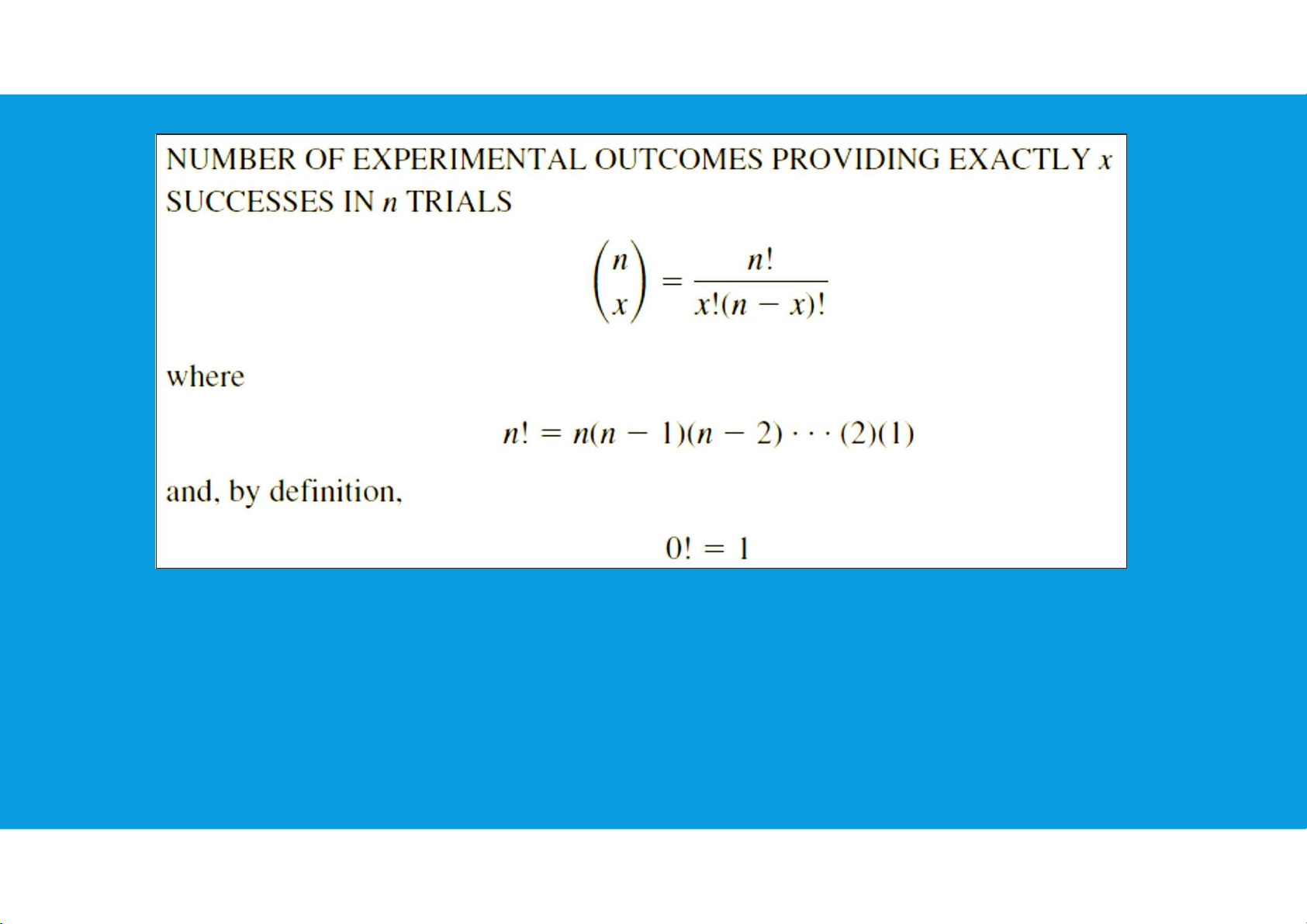
Combinations: allows one to count the number of experimental outcomes when the
experiment involves selecting n objects from a set of N objects.
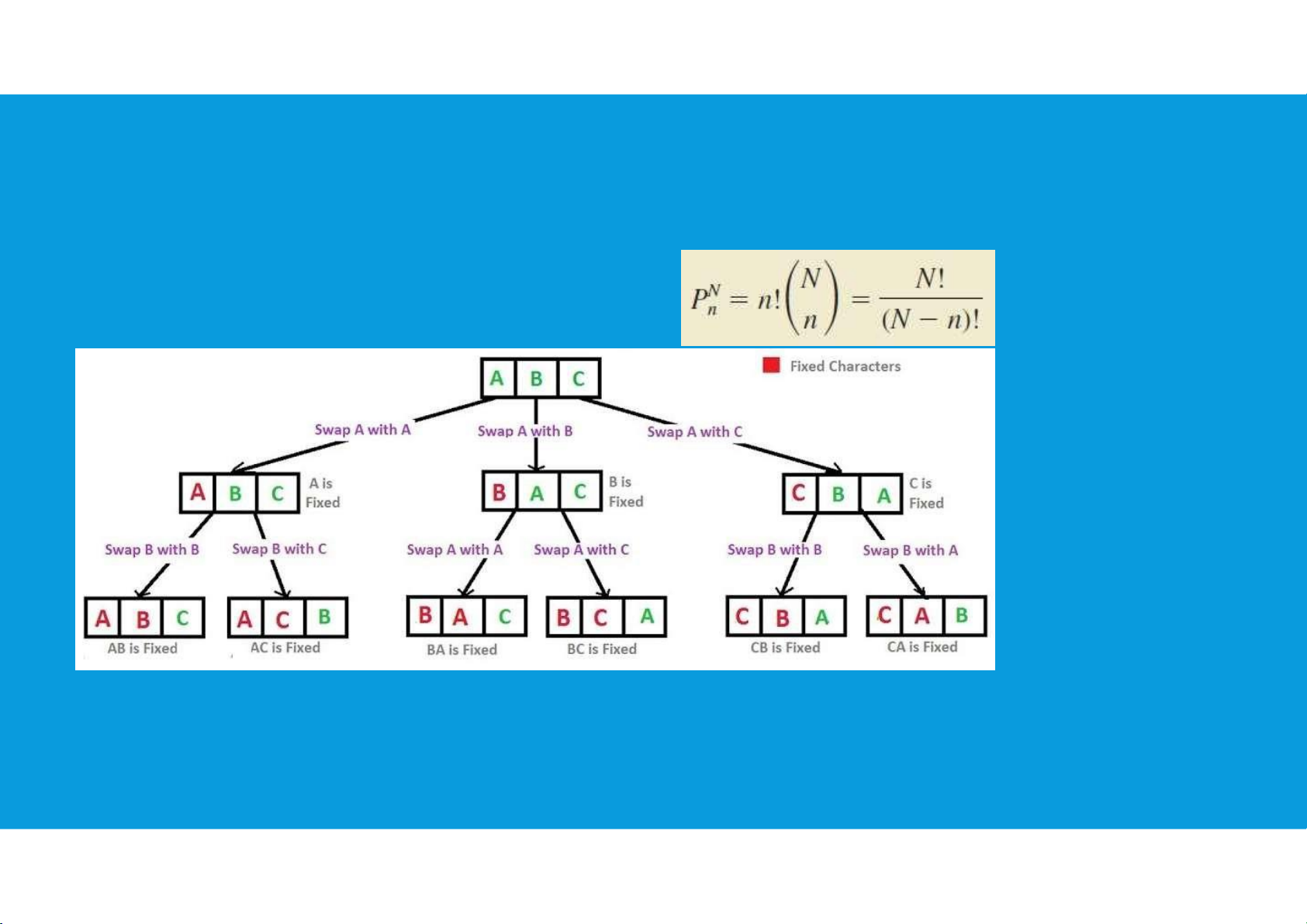
The notation ! means factorial; for example, 5 factorial is 5! = (5)(4)(3)(2)(1) = 120 4.1. INTRODUCTION TO PROBABILITY •Counting rules: Permutations: allows one to compute the number of tttu@hcmiu.edu.vn 7 lOMoARcPSD|364 906 32
experimental outcomes when n objects are to be selected from a set of N objects
where the order of selection is important. The same n objects selected in a different
order are considered a different experimental outcome. tttu@hcmiu.edu.vn 8 lOMoARcPSD|364 906 32
4.1. INTRODUCTION TO PROBABILITY •Assigning probabilities:
The three approaches most frequently used are the classical, relative frequency, and subjective methods.
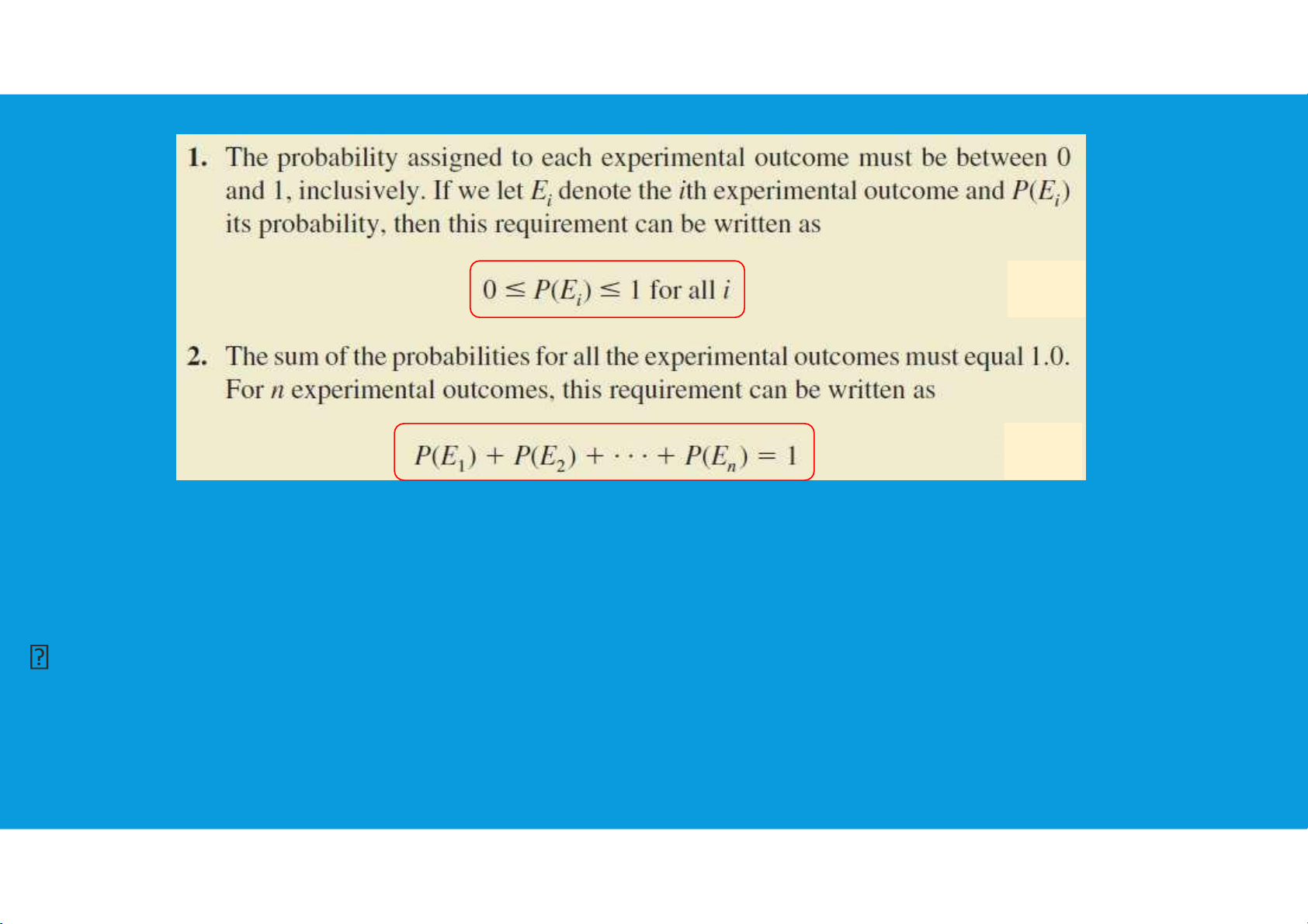
Regardless of the method used, two basic requirements for assigning probabilities must be met. tttu@hcmiu.edu.vn 9 lOMoARcPSD|364 906 32
4.1. INTRODUCTION TO PROBABILITY •Assigning probabilities:
The classical method of assigning probabilities is appropriate when all the
experimental outcomes are equally likely. tttu@hcmiu.edu.vn 10 lOMoARcPSD|364 906 32
When using this approach, the two basic requirements for assigning
probabilities are automatically satisfied.
If n experimental outcomes are possible,
a probability of 1/n is assigned to each experimental outcome
4.1. INTRODUCTION TO PROBABILITY •Assigning probabilities:
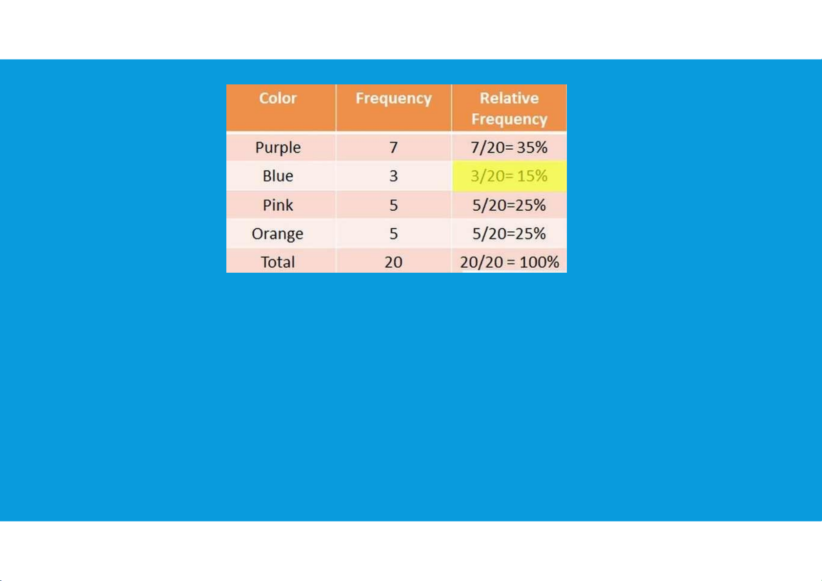
The relative frequency method of assigning probabilities is appropriate when data
are available to estimate the proportion of the time the experimental outcome will
occur if the experiment is repeated a large number of times. tttu@hcmiu.edu.vn 11 lOMoARcPSD|364 906 32
When using this approach, the two basic requirements for assigning probabilities are automatically satisfied.
4.1. INTRODUCTION TO PROBABILITY •Assigning probabilities: tttu@hcmiu.edu.vn 12 lOMoARcPSD|364 906 32
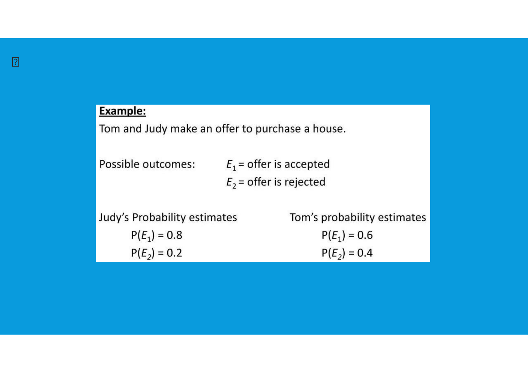
The subjective method of assigning probabilities is most appropriate when one
cannot realistically assume that the experimental outcomes are equally likely and
when little relevant data are available.
4.1. INTRODUCTION TO PROBABILITY
•Events and their probabilities: tttu@hcmiu.edu.vn 13 lOMoARcPSD|364 906 32
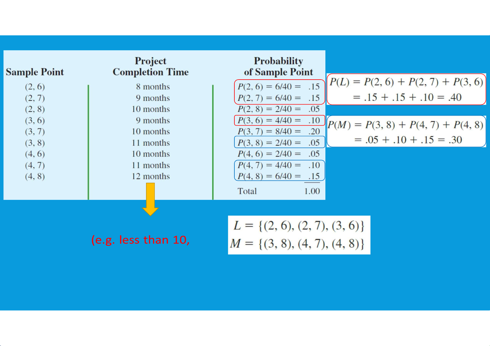
An event is a collection of sample points.
The probability of any event is equal to the sum of the probabilities of the sample points in the event.
calculate the probability of a particular event by adding the probabilities of the
sample points (experimental outcomes) that make up the event.
4.1. INTRODUCTION TO PROBABILITY
•Events and their probabilities: tttu@hcmiu.edu.vn 14 lOMoARcPSD|364 906 32 Events equal 10, more than 10, etc.) tttu@hcmiu.edu.vn 15 lOMoARcPSD|364 906 32
4.1. INTRODUCTION TO PROBABILITY
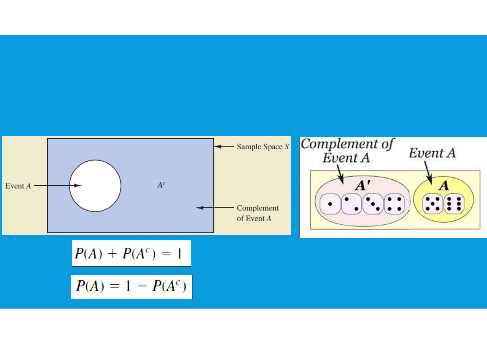
•Some basic relationships of probability: tttu@hcmiu.edu.vn 16 lOMoARcPSD|364 906 32
The complement of A is defined to be the event consisting of all sample points
that are not in A. The complement of a is denoted by Ac. tttu@hcmiu.edu.vn 17 lOMoARcPSD|364 906 32
4.1. INTRODUCTION TO PROBABILITY
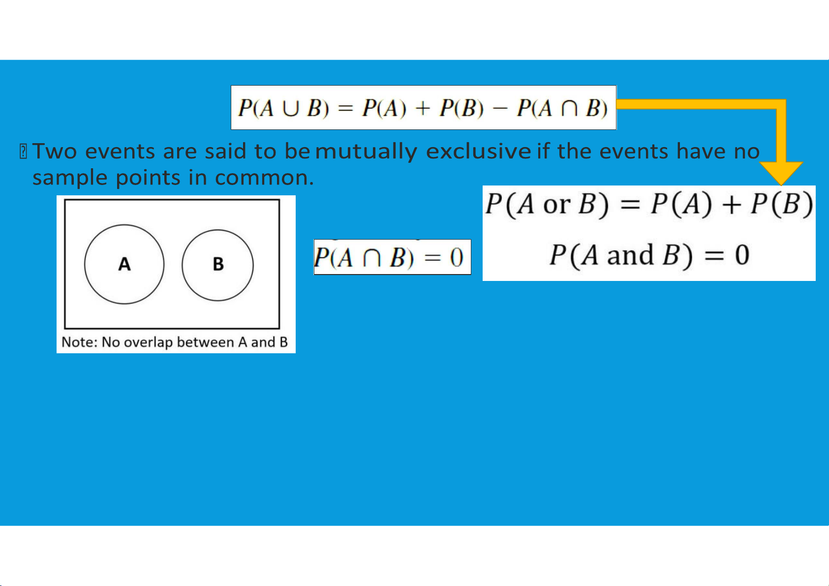
•Some basic relationships of probability:
Addition Law: is helpful when we are interested in knowing the probability that
at least one of two events occurs. That is, with events A and B we are interested
in knowing the probability that event A or event B or both occur.
Addition Law: two concepts related to the combination of events: the union of
events and the intersection of events.
-The union of A and B is the event containing all
-The intersection of A and B is the event containing
sample points belonging to A or B or both. The
the sample points belonging to both A and B. The union is denoted by A U B.
intersection is denoted by A ∩ B. tttu@hcmiu.edu.vn 18 lOMoARcPSD|364 906 32
4.1. INTRODUCTION TO PROBABILITY
•Some basic relationships of probability:
The addition law provides a way to compute the probability that event A or
event B or both occur. In other words, the addition law is used to compute the
probability of the union of two events. tttu@hcmiu.edu.vn 19 lOMoARcPSD|364 906 32
4.1. INTRODUCTION TO PROBABILITY
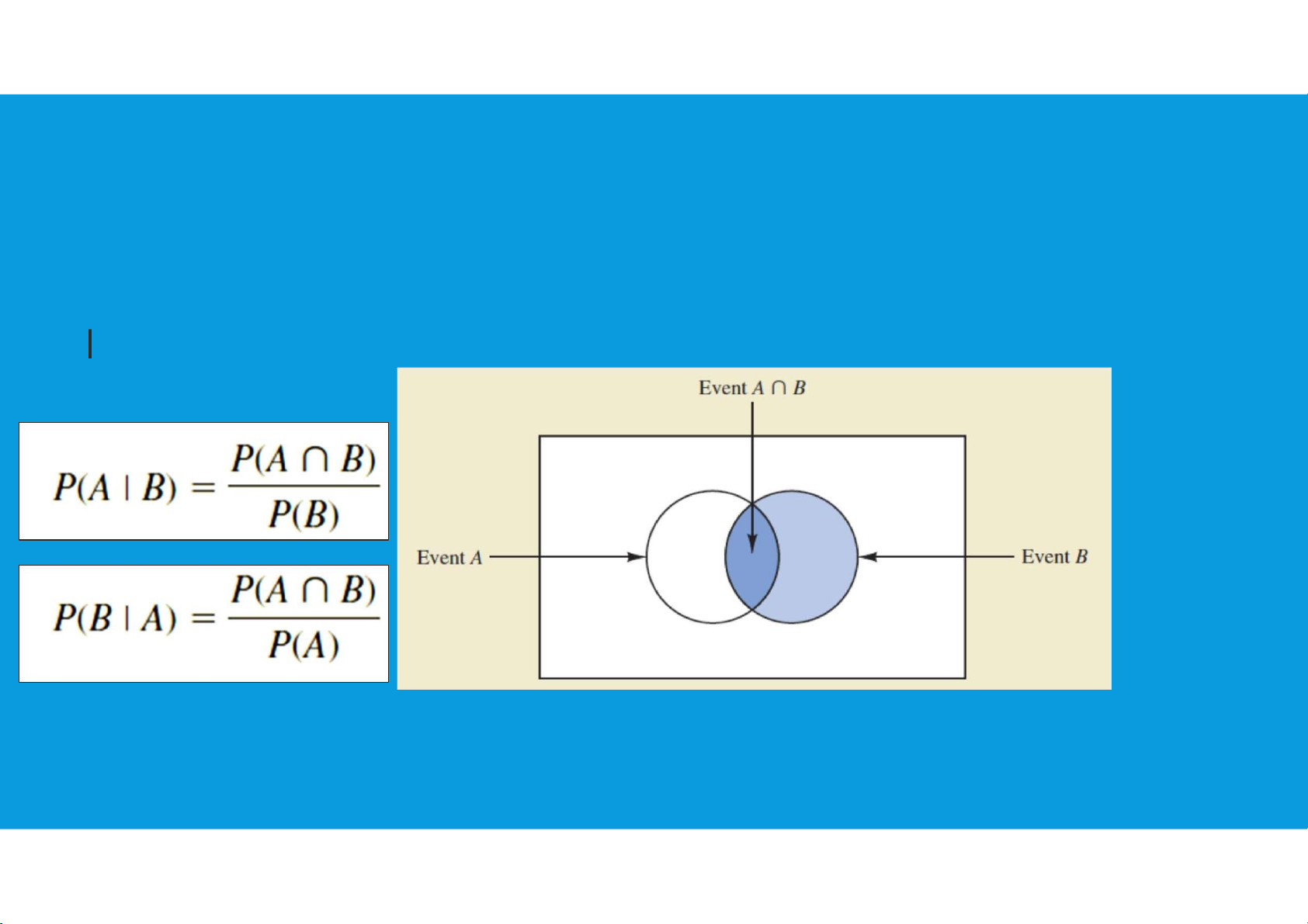
•Conditional probability: Suppose we have an event A with tttu@hcmiu.edu.vn 20 lOMoARcPSD|364 906 32
probability P(A). If we obtain new information and learn that A related event,
denoted by B, already occurred, we will want to take advantage of this
information by calculating a new probability for event A.
•This new probability of event A is called a conditional probability and is written
P(A B) (“the probability of A given B”)
4.1. INTRODUCTION TO PROBABILITY tttu@hcmiu.edu.vn 21 lOMoARcPSD|364 906 32 tttu@hcmiu.edu.vn 22 lOMoARcPSD|364 906 32
4.1. INTRODUCTION TO PROBABILITY tttu@hcmiu.edu.vn 23 lOMoARcPSD|364 906 32
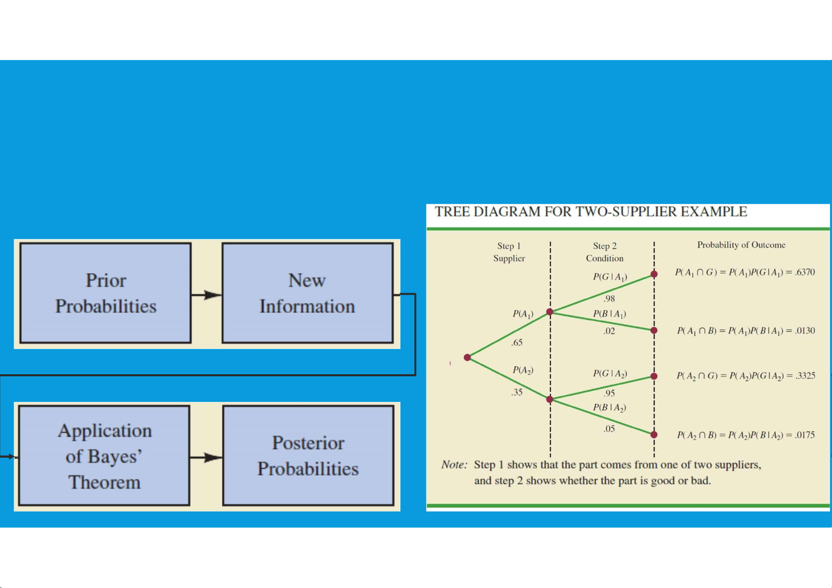
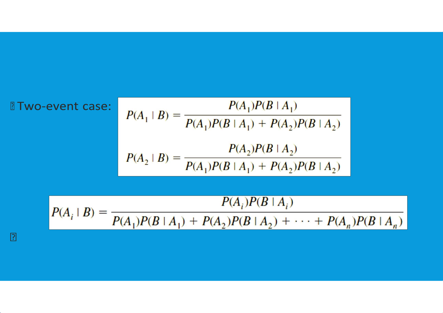
•Bayes’ theorem: is applied when probability revision is needed
(new information for the events occur) tttu@hcmiu.edu.vn 24 lOMoARcPSD|364 906 32
4.1. INTRODUCTION TO PROBABILITY •Bayes’ theorem: n mutually exclusive case: tttu@hcmiu.edu.vn 25 lOMoARcPSD|364 906 32 End of file 1. Any questions? tttu@hcmiu.edu.vn 22
4.2. DISCRETE PROBABILITY DISTRIBUTIONS •Random variables
•Developing discrete probability distributions
•Bivariate distributions, covariance, and financial portfolios lOMoARcPSD|364 906 32
•Binomial probability distribution
•Poisson probability distribution
•Hypergeometric probability distribution
4.2. DISCRETE PROBABILITY DISTRIBUTIONS
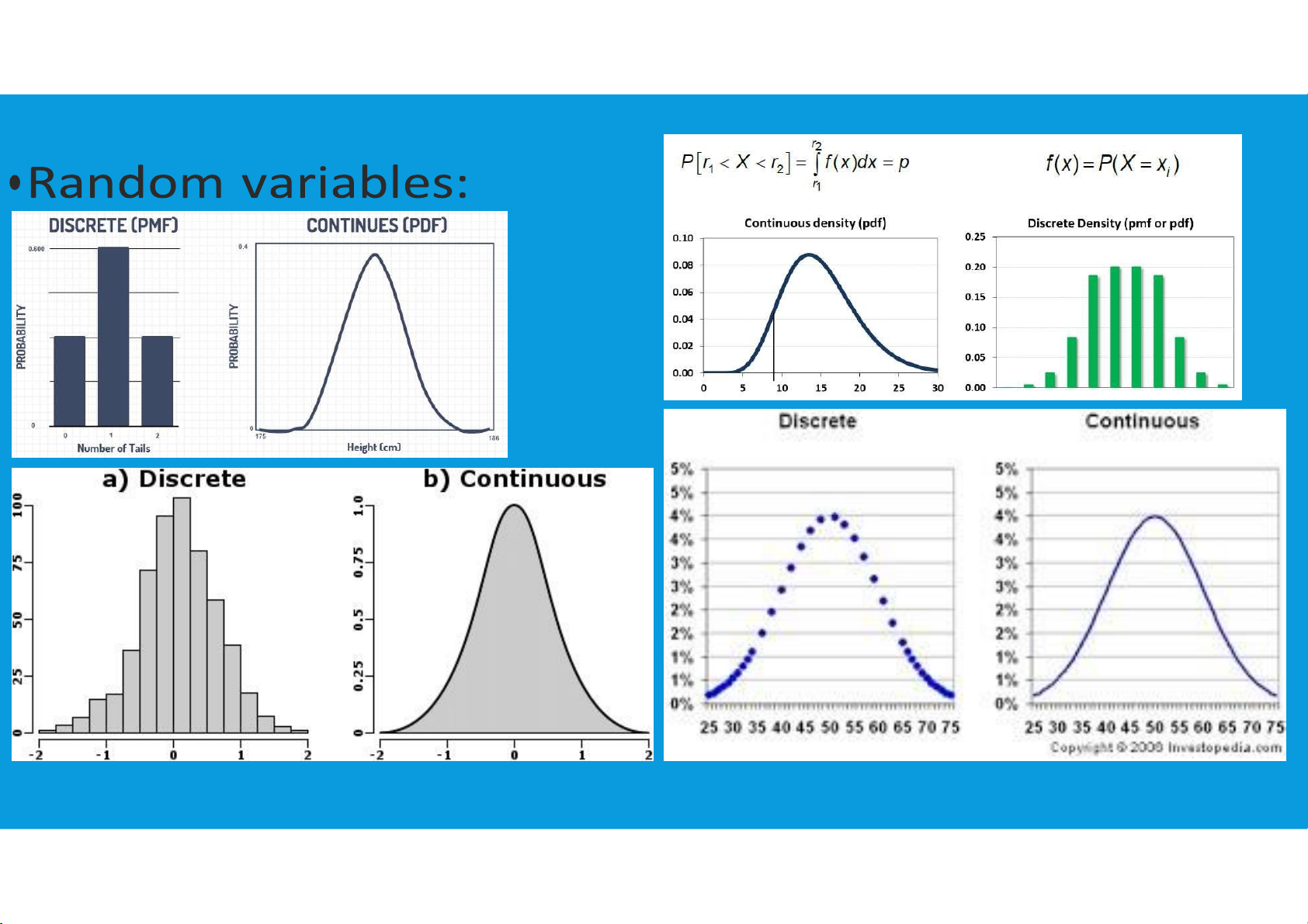
•Random variables: numerical description of the outcome of an experiment. Discrete Random Variables:
A random variable that may assume either a finite number of values or an
infinite sequence of values such as 0, 1, 2, . . . is referred to as a discrete random variable. tttu@hcmiu.edu.vn 27 lOMoARcPSD|364 906 32
4.2. DISCRETE PROBABILITY DISTRIBUTIONS
•Random variables: numerical description of the outcome of an experiment.
Continuous Random Variables: A random variable that may assume any
numerical value in an interval or collection of intervals is called a continuous
random variable. Experimental outcomes based on measurement scales such as tttu@hcmiu.edu.vn 28 lOMoARcPSD|364 906 32
time, weight, distance, and temperature can be described by continuous random variables.
4.2. DISCRETE PROBABILITY DISTRIBUTIONS tttu@hcmiu.edu.vn 29 lOMoARcPSD|364 906 32 tttu@hcmiu.edu.vn 30 lOMoARcPSD|364 906 32
4.2. DISCRETE PROBABILITY DISTRIBUTIONS
•Developing discrete probability distributions:
•The probability distribution for a random variable describes how probabilities are
distributed over the values of the random variable.
•For a discrete random variable x, a probability function, denoted by f(x), provides
the probability for each value of the random variable.
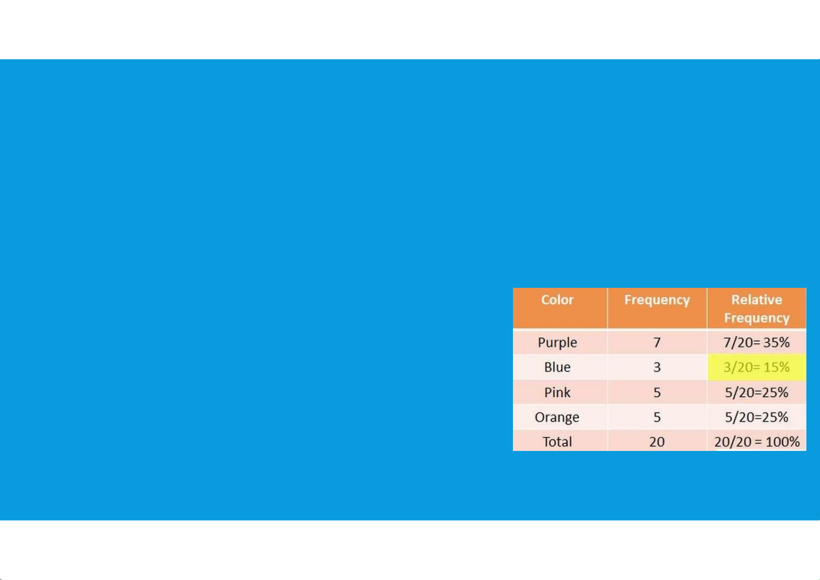
•The relative frequency method of assigning probabilities to values of a random
variable is applicable when reasonably large amounts of data are available.
•We then treat the data as if they were the population and use the relative
frequency method to assign probabilities to the experimental outcomes.
•The use of the relative frequency method to develop discrete probability
distributions leads to what is called an empirical discrete distribution. tttu@hcmiu.edu.vn 31 lOMoARcPSD|364 906 32
4.2. DISCRETE PROBABILITY DISTRIBUTIONS
•Developing discrete probability distributions:
A primary advantage of defining a random variable and its probability
distribution is that once the probability distribution is known, it is relatively easy
to determine the probability of a variety of events that may be of interest to a decision maker.
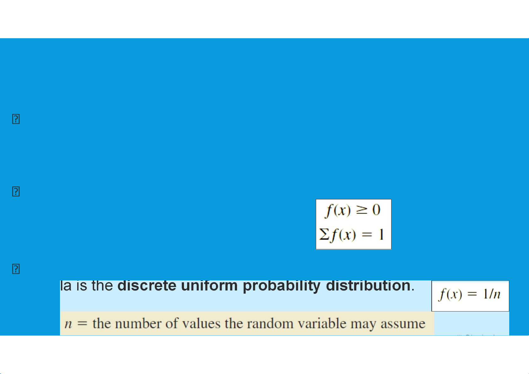
In the development of a probability function for any discrete random variable,
the following two conditions must be satisfied.
The simplest example of a discrete probability distribution given by a formula is
the discrete uniform probability distribution.
4.2. DISCRETE PROBABILITY DISTRIBUTIONS tttu@hcmiu.edu.vn 32 lOMoARcPSD|364 906 32
•Developing discrete probability distributions:
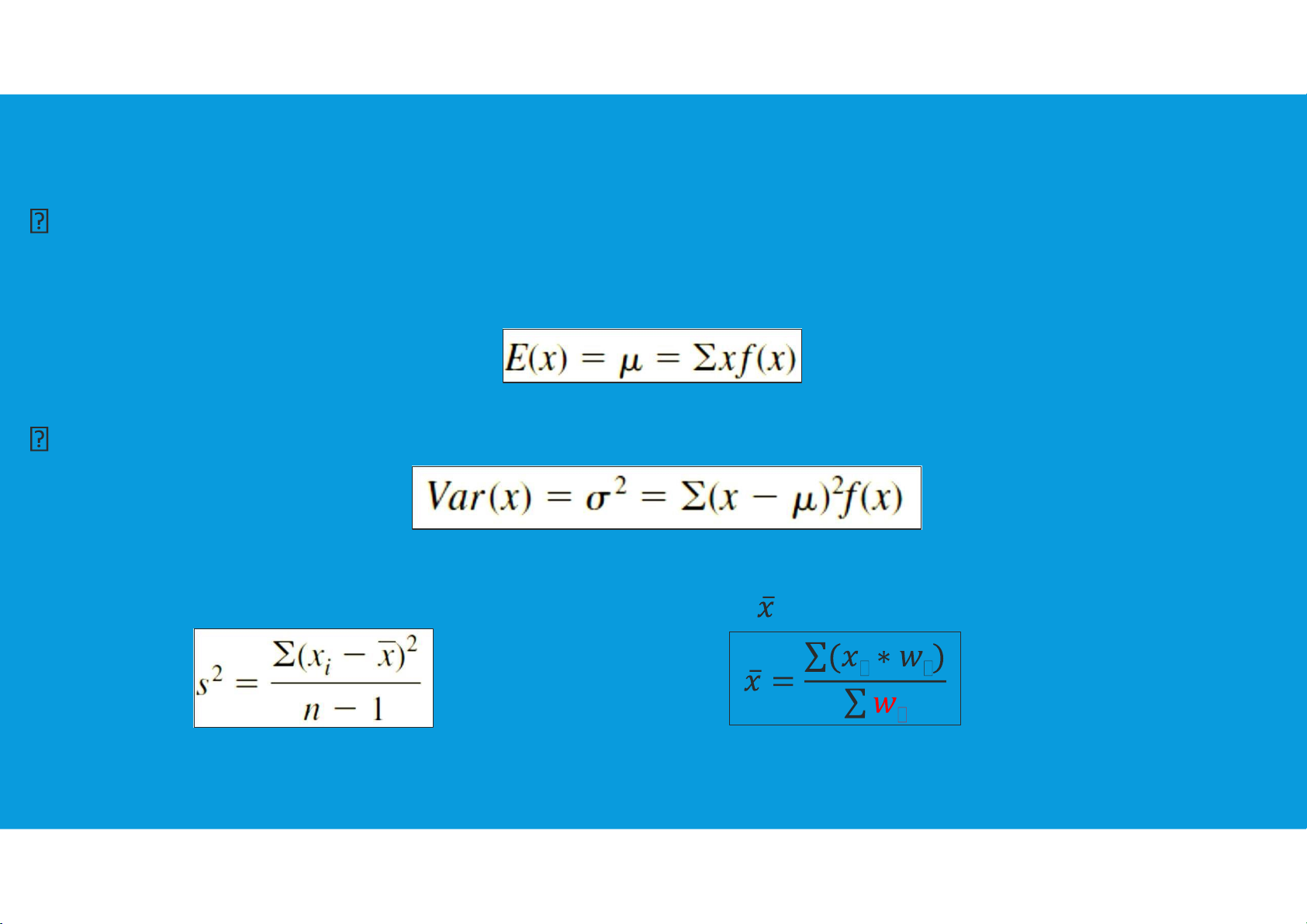
Expected value: or mean, of a random variable is a measure of the central
location for the random variable. The formula for the expected value of a
discrete random variable x follows.
Variance: summarize the variability in the values of a random variable
Recall (Lecture4): Sample variance
In which, : mean (or weighted mean)
4.2. DISCRETE PROBABILITY DISTRIBUTIONS tttu@hcmiu.edu.vn 33 lOMoARcPSD|364 906 32
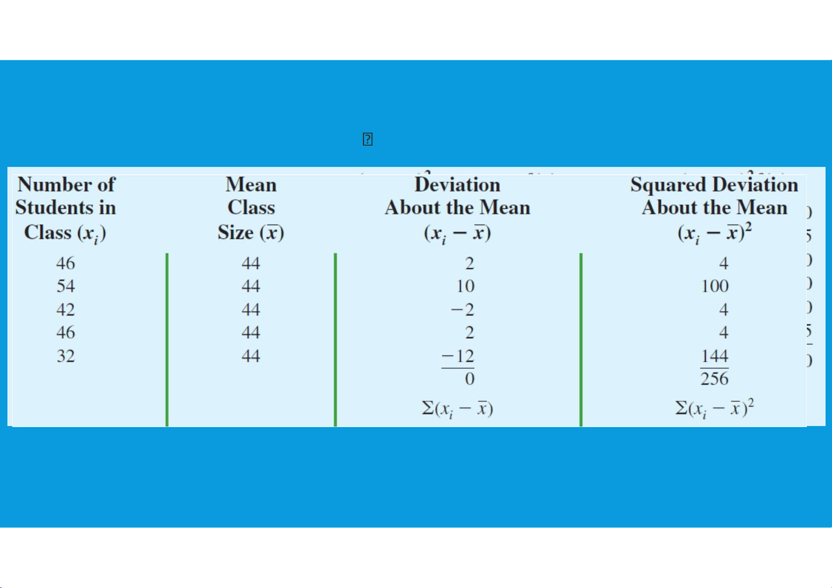
•Developing discrete probability distributions:
•Recall (Lecture4): Variance Variance:= 256/4= 64
4.2. DISCRETE PROBABILITY DISTRIBUTIONS tttu@hcmiu.edu.vn 34 lOMoARcPSD|364 906 32
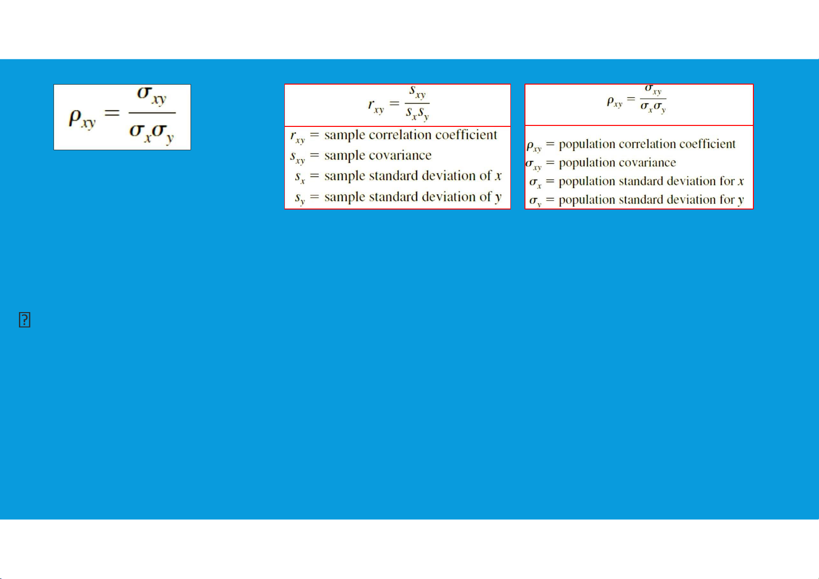
•Bivariate distributions, covariance, correlation:
A probability distribution involving two random variables is called a
bivariate probability distribution. Recall (Lecture5) Covariance of random variables x and y:
Correlation of random variables x and y: tttu@hcmiu.edu.vn 35 lOMoARcPSD|364 906 32
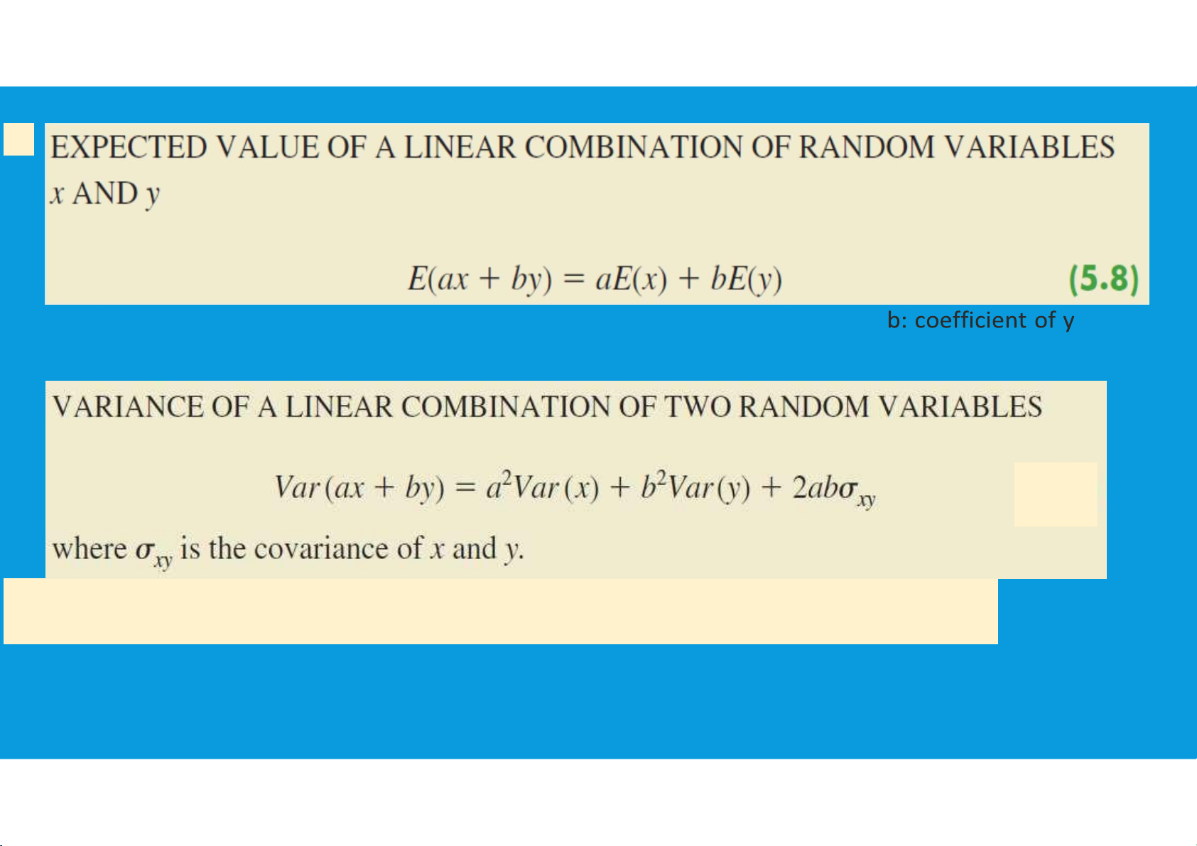
4.2. DISCRETE PROBABILITY DISTRIBUTIONS
•Bivariate distributions, covariance, correlation:
Linear combination of random variables x and y tttu@hcmiu.edu.vn 36 lOMoARcPSD|364 906 32 In which: a: coefficient of x
4.2. DISCRETE PROBABILITY DISTRIBUTIONS tttu@hcmiu.edu.vn 37 lOMoARcPSD|364 906 32
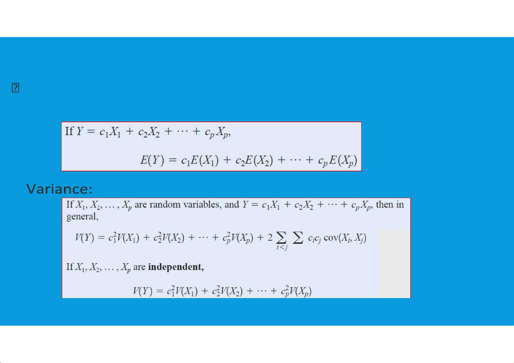
•Bivariate distributions, covariance, correlation:
Linear combination of p random variables Expected value: tttu@hcmiu.edu.vn 38 lOMoARcPSD|364 906 32 tttu@hcmiu.edu.vn 39 lOMoARcPSD|364 906 32
4.2. DISCRETE PROBABILITY DISTRIBUTIONS
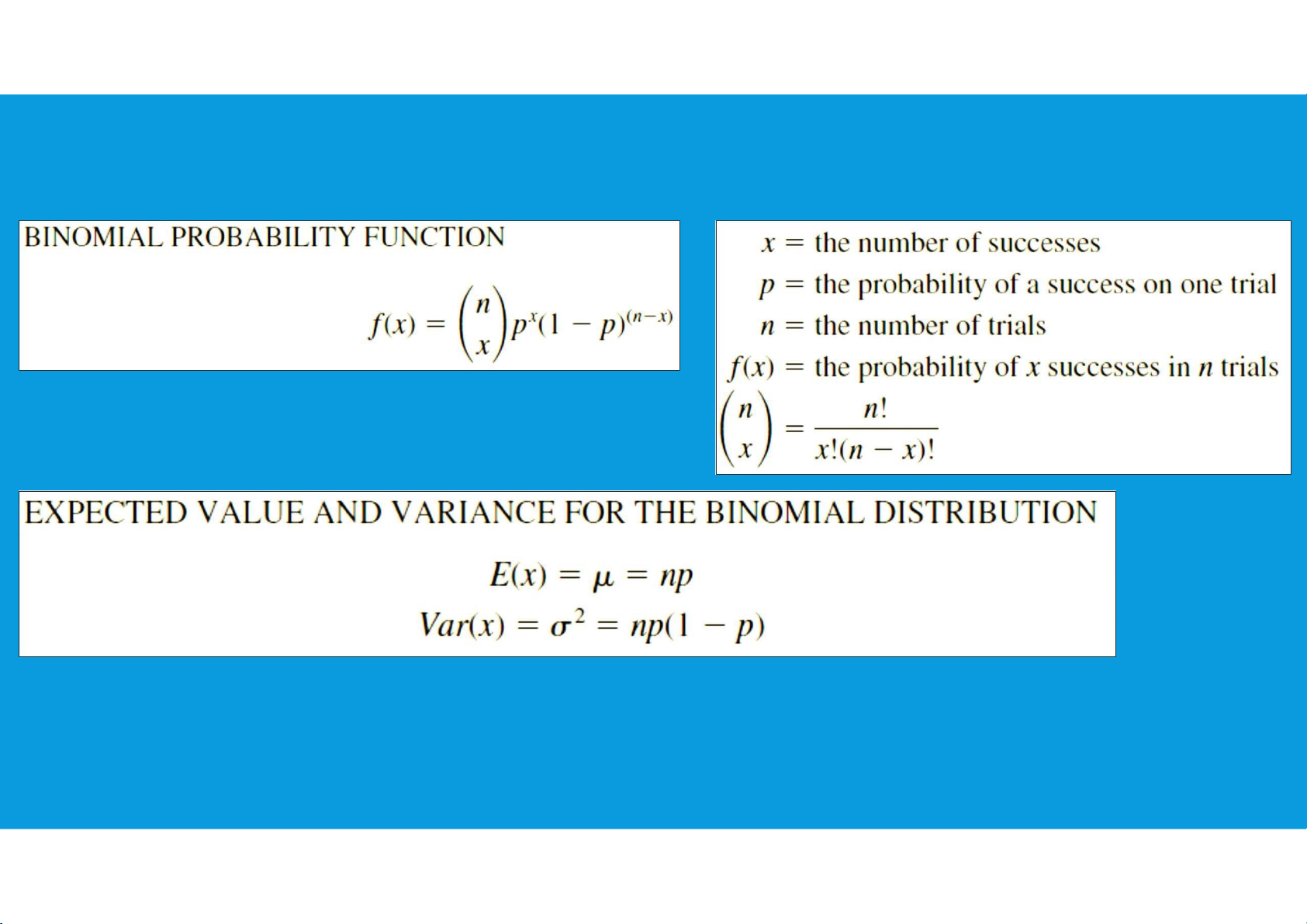
•Binomial probability distribution: The probability distribution
associated with this random variable is called the binomial probability distribution. tttu@hcmiu.edu.vn 40 lOMoARcPSD|364 906 32
4.2. DISCRETE PROBABILITY DISTRIBUTIONS
•Binomial probability distribution: for the binomial probability tttu@hcmiu.edu.vn 41 lOMoARcPSD|364 906 32
distribution, x is a discrete random variable with the probability function f(x)
applicable for values of x = 0, 1, 2, . . . , n. tttu@hcmiu.edu.vn 42 lOMoARcPSD|364 906 32
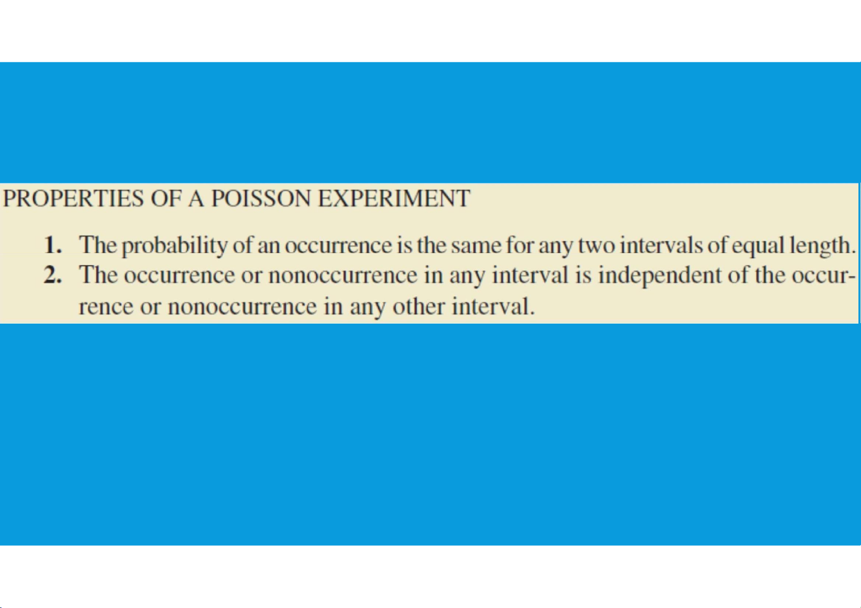
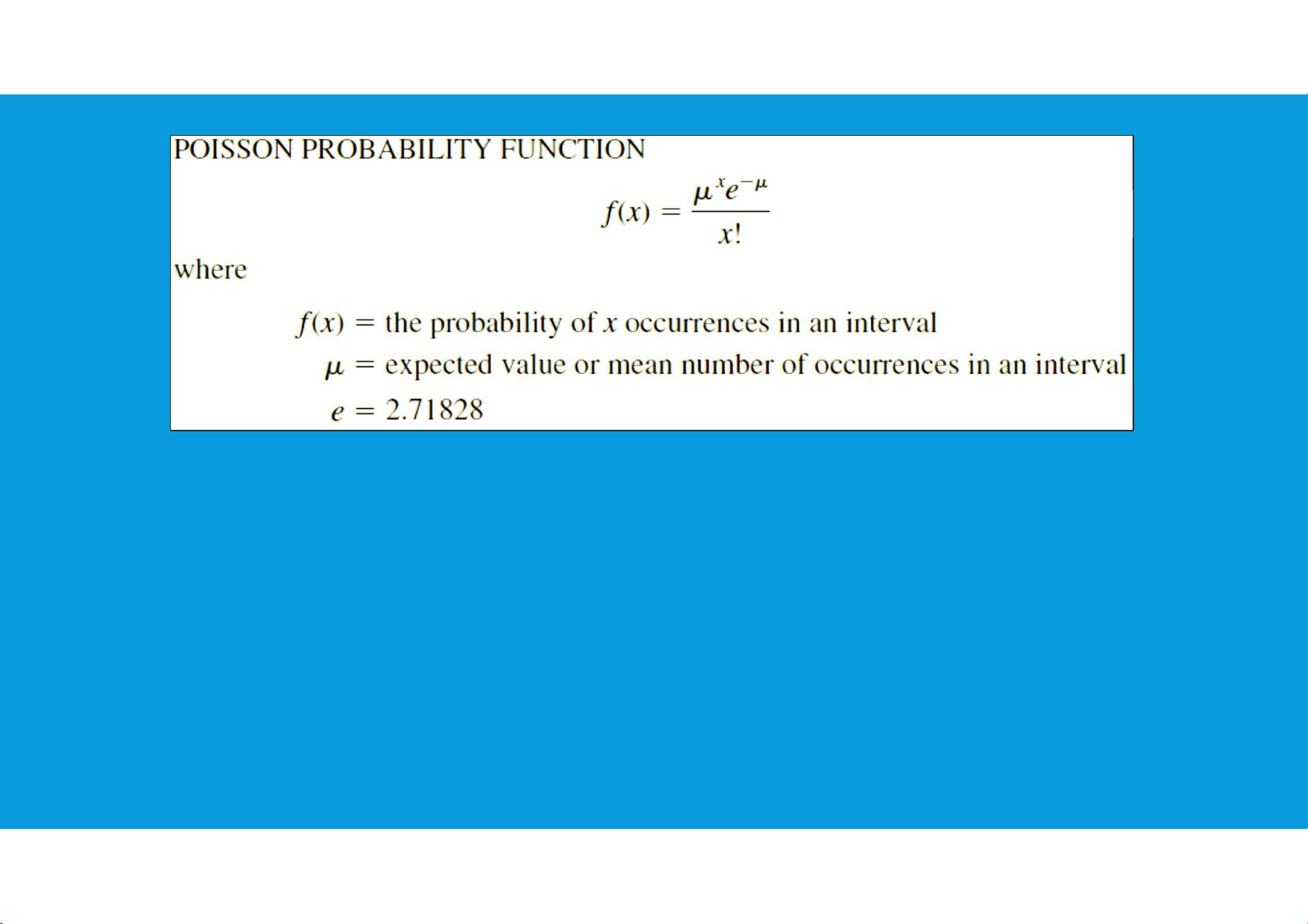
4.2. DISCRETE PROBABILITY DISTRIBUTIONS •Poisson probability distribution: tttu@hcmiu.edu.vn 43 lOMoARcPSD|364 906 32
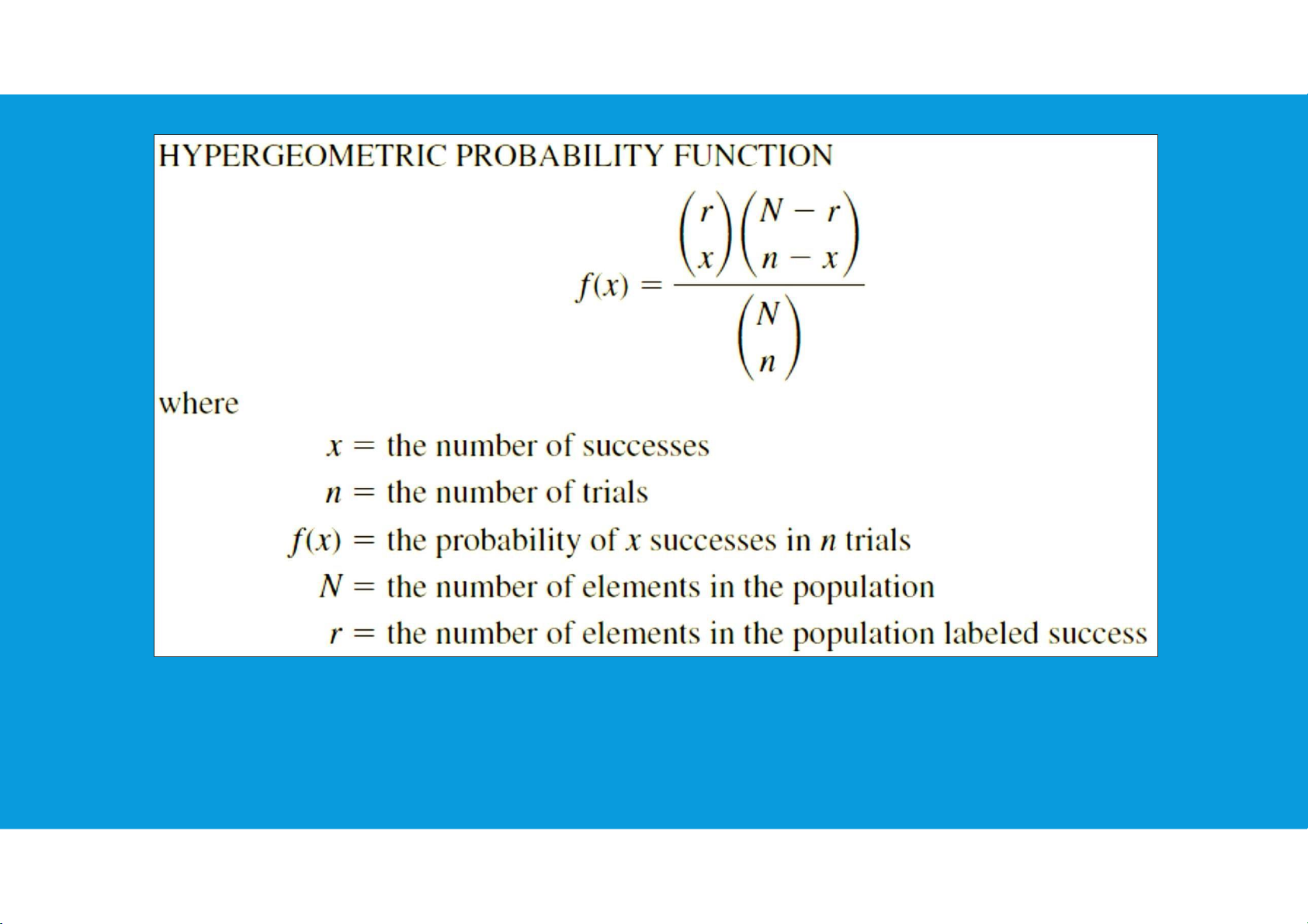
4.2. DISCRETE PROBABILITY DISTRIBUTIONS •Hypergeometric probability distribution: tttu@hcmiu.edu.vn 44 lOMoARcPSD|364 906 32 tttu@hcmiu.edu.vn 45 lOMoARcPSD|364 906 32 End of file 2. Any questions? tttu@hcmiu.edu.vn 39
Document Outline

• APPLIED STATISTICS
  • Chapter 4: Probability and Distribution