Lecture Notes 1: Introduction to Graph Theory Concepts | Toán Rời Rạc | Trường Đại học Khoa học Tự nhiên, Đại học Quốc gia Hà Nội
First suppose we have a graph G in which any two vertices are connected by a unique path. Then G is certainly connected. Moreover, if G contained a cycle v1 . . .vkv1, then v1vk and v1v2 · · · vk would be two distinct paths between v1 and vk. Hence G is a tree. Suppose G is a tree and u, v ∈ V (G). Since G is connected, there is at least one path from u to v. Suppose there are two distinct paths P, P 0 from u to v. If these paths only intersect at u and v, we can immediately combine them into a cycle, but in general the paths could. Tài liệu được sưu tầm và soạn thảo dưới dạng file PDF để gửi tới các bạn cùng tham khảo, ôn tập đầy đủ kiến thức, chuẩn bị cho các buổi học thật tốt. Mời bạn đọc đón xem!
Môn: Toán Rời Rạc (HUS) 11 tài liệu
Trường: Trường Đại học Khoa học tự nhiên, Đại học Quốc gia Hà Nội 1.1 K tài liệu
Tác giả:
Preview text:
Graph Theory 2018 – EPFL – Lecture Notes. Lecturer: D´ aniel Kor´ andi May 31, 2018
Acknowledgements: These notes are partially based on the lecture notes of the Graph
Theory courses given by Frank de Zeeuw and Andrey Kupavskii. Lecture 1 Introduction 1 Definitions
Definition. A graph G = (V, E) consists of a finite set V and a set E of two-element subsets
of V . The elements of V are called vertices and the elements of E are called edges.
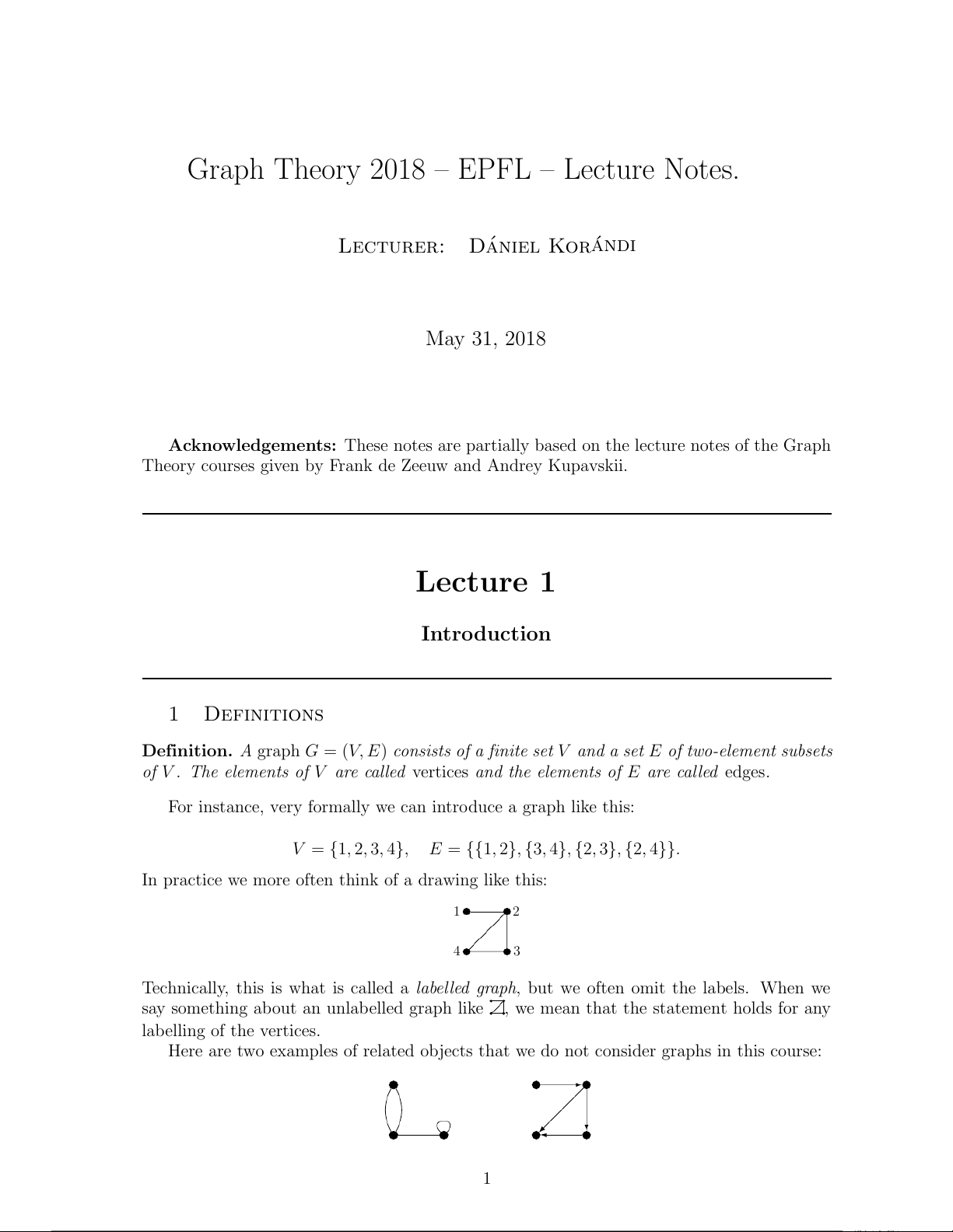
For instance, very formally we can introduce a graph like this:
V = {1, 2, 3, 4}, E = {{1, 2}, {3, 4}, {2, 3}, {2, 4}}.
In practice we more often think of a drawing like this: 1 2 4 3
Technically, this is what is called a labelled graph, but we often omit the labels. When we
say something about an unlabelled graph like
, we mean that the statement holds for any labelling of the vertices.
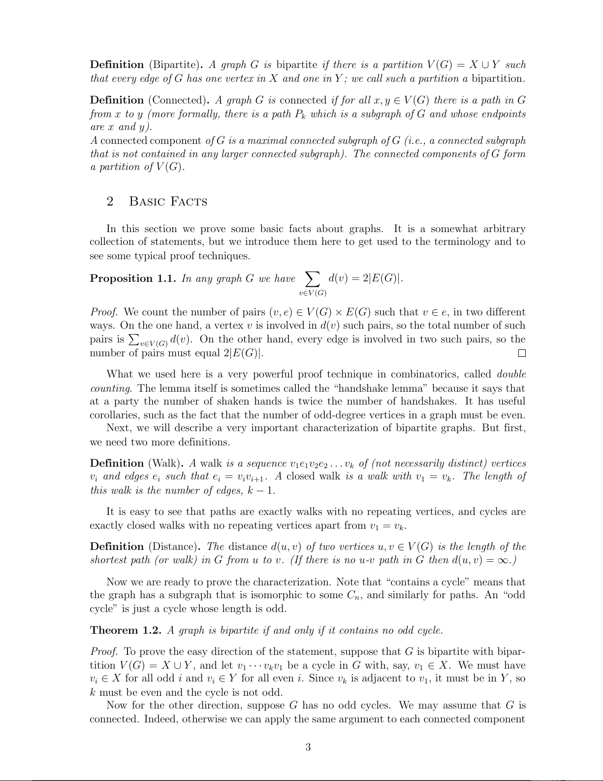
Here are two examples of related objects that we do not consider graphs in this course: 1
The first is a multigraph, which can have multiple edges and loops; the corresponding defini-
tion would allow the edge set and the edges to be multisets. The second is a directed graph, in
which every edge has a direction; in the corresponding definition the edges would be ordered
pairs instead of two-element subsets.
Although this course is mostly not about these variants, in some cases it will be more
natural to state our results for directed or multigraphs. In any case, we will not treat infinite graphs in this course.
Graphs (and their above-mentioned variants) are highly applicable in- and outside math-
ematics because they provide a simple way of modeling many concepts involving connec-
tions between objects. For example, graphs can model social networks (vertices=people &
edges=friendships), computer networks (computers & links), molecules (atoms & bonds) and
many other things. The aim of this course is to study graphs in the abstract sense, and to
introduce the fundamental concepts, tools, tricks and results about them.
Some notation: Given a graph G, we write V (G) for the vertex set, and E(G) for the
edge set. For an edge {x, y} ∈ E(G), we usually write xy, and we consider yx to be the same
edge. If xy ∈ E(G), then we say that x, y ∈ V (G) are adjacent or connected or that they are
neighbors. If x ∈ e, then we say that x ∈ V (G) and e ∈ E(G) are incident.
Definition (Subgraphs). Two graphs G, G0 are isomorphic if there is a bijection ϕ : V (G) →
V (G0) such that xy ∈ E(G) if and only if ϕ(x)ϕ(y) ∈ E(G0). A graph H is a subgraph of a
graph G, denoted H ⊂ G, if there is a graph H0 isomorphic to H such that V (H0) ⊂ V (G) and E(H0) ⊂ E(G).
With this definition we can for instance say that is a subgraph of . As mentioned
above, when we talk about graphs we often omit the labels of the vertices. A more formal way
of doing this is to define an unlabelled graph to be an isomorphism class of labelled graphs.
We will be somewhat informal about this distinction, since it rarely leads to confusion.
Definition (Degree). Fix a graph G = (V, E). For v ∈ V , we write N (v) = {w ∈ V : vw ∈ E}
for the set of neighbors of v (which does not include v). Then d(v) = |N(v)| is the degree
of v. We write δ(G) for the minimum degree of a vertex in G, and ∆(G) for the maximum degree.
Definition (Examples). The following are some of the most common types of graphs.
• Paths are the graphs Pn of the form
. The graph Pn has n − 1 edges and n
different vertices; we say that Pn has length n − 1.
• Cycles are the graphs Cn of the form
. The graph Cn has n edges and n
different vertices; the length of Cn is defined to be n.
• Complete graphs (or cliques) are the graphs Kn on n vertices in which all vertices are adjacent. The graph K n has n edges. For instance, K 2 4 is .
• The complete bipartite graphs are the graphs Ks,t with a partition V (Ks,t) = X ∪ Y
with |X| = s, |Y | = t, such that every vertex of X is adjacent to every vertex of Y , and
there are no edges inside X or Y . Then Kst has st edges. For example, K2,3 is .
The following are the most common properties of graphs that we will consider. 2
Definition (Bipartite). A graph G is bipartite if there is a partition V (G) = X ∪ Y such
that every edge of G has one vertex in X and one in Y ; we call such a partition a bipartition.
Definition (Connected). A graph G is connected if for all x, y ∈ V (G) there is a path in G
from x to y (more formally, there is a path Pk which is a subgraph of G and whose endpoints are x and y).
A connected component of G is a maximal connected subgraph of G (i.e., a connected subgraph
that is not contained in any larger connected subgraph). The connected components of G form a partition of V (G). 2 Basic Facts
In this section we prove some basic facts about graphs. It is a somewhat arbitrary
collection of statements, but we introduce them here to get used to the terminology and to
see some typical proof techniques. X
Proposition 1.1. In any graph G we have d(v) = 2|E(G)|. v∈V (G)
Proof. We count the number of pairs (v, e) ∈ V (G) × E(G) such that v ∈ e, in two different
ways. On the one hand, a vertex v is involved in d(v) such pairs, so the total number of such pairs is P
d(v). On the other hand, every edge is involved in two such pairs, so the v∈V (G)
number of pairs must equal 2|E(G)|.
What we used here is a very powerful proof technique in combinatorics, called double
counting. The lemma itself is sometimes called the “handshake lemma” because it says that
at a party the number of shaken hands is twice the number of handshakes. It has useful
corollaries, such as the fact that the number of odd-degree vertices in a graph must be even.
Next, we will describe a very important characterization of bipartite graphs. But first, we need two more definitions.
Definition (Walk). A walk is a sequence v1e1v2e2 . . . vk of (not necessarily distinct) vertices
vi and edges ei such that ei = vivi+1. A closed walk is a walk with v1 = vk. The length of
this walk is the number of edges, k − 1.
It is easy to see that paths are exactly walks with no repeating vertices, and cycles are
exactly closed walks with no repeating vertices apart from v1 = vk.
Definition (Distance). The distance d(u, v) of two vertices u, v ∈ V (G) is the length of the
shortest path (or walk) in G from u to v. (If there is no u-v path in G then d(u, v) = ∞.)
Now we are ready to prove the characterization. Note that “contains a cycle” means that
the graph has a subgraph that is isomorphic to some Cn, and similarly for paths. An “odd
cycle” is just a cycle whose length is odd.
Theorem 1.2. A graph is bipartite if and only if it contains no odd cycle.
Proof. To prove the easy direction of the statement, suppose that G is bipartite with bipar-
tition V (G) = X ∪ Y , and let v1 · · · vkv1 be a cycle in G with, say, v1 ∈ X. We must have
vi ∈ X for all odd i and vi ∈ Y for all even i. Since vk is adjacent to v1, it must be in Y , so
k must be even and the cycle is not odd.
Now for the other direction, suppose G has no odd cycles. We may assume that G is
connected. Indeed, otherwise we can apply the same argument to each connected component 3
Gi of G to get a bipartition Xi ∪ Yi of Gi. Choosing X = ∪iXi and Y = ∪iYi will then give a bipartition of G.
So if v is a fixed vertex, then every other vertex u ∈ V (G) has finite distance from v. Let
X = {u : distance of v and u is even}
Y = {u : distance of v and u is odd }.
Our aim is to prove that this is a bipartition of G. For this, we need to check that no two
vertices in X are adjacent and no two vertices in Y are adjacent.
Suppose for contradiction that some two vertices u1, u2 ∈ X are adjacent, and let e be
the edge u1u2. By construction, there are paths P1 from v to u1 and P2 from u2 to v that
both have even lengths. But then joining P1, P2 and the edge e gives a closed walk P1eP2
of odd length, so by Claim 1.3 below, G contains an odd cycle, as well, contradiction the
assumption. (Note that P1eP2 is not necessarily a cycle because P1 and P2 might intersect!)
We can do the same to show that no two vertices u1, u2 ∈ Y are adjacent: here the paths
P1, P2 will both have odd lengths, so again P1eP2 is a closed odd walk. So X ∪ Y is indeed a bipartition of G.
The proof above is a constructive argument, where we explicitly constructed the object
we were looking for (and then proved that it satisfies the required properties). Of course, we
still need to prove the following lemma to complete the proof. We use an inductive argument.
Claim 1.3. Every closed walk of odd length contains an odd cycle.
Proof. We apply induction on the length k of the walk. Since there is no closed walk of
length 1, the statement is vacuously true for k = 1. We could use this as the base case, but
it is also easy to see that the only closed walk of length 3 is the triangle (K3), which itself is an odd cycle.
Now suppose the statement is true for every odd length < k, and let W = v1e1v2 . . . vk+1
be a closed walk of odd length k. Let j be the smallest index such that vi = vj for some
i < j. We have two cases. If j − i is even, then deleting the j − i edges ei, . . . , ej−1 from W
yields another closed walk W 0 ⊆ W of odd length. Applying induction on W 0 then gives an
odd cycle in W 0 and hence in W .
On the other hand, if j − i is odd (and it cannot be 1, so j − i ≥ 3), then the j − i edges
ei, . . . , ej−1 form an odd cycle. Indeed, they form an odd walk without repeated vertices by
the choice of vj. This is what we were looking for.
The next lemma shows that if all degrees of a graph are large, then it must contain a
long path. The proof is an example of an extremal argument, where we take an object that is
extremal with respect to some property, and show that this extremality implies some other property of the object.
Proposition 1.4. A graph G with minimum degree δ(G) contains a path of length at least δ(G).
Proof. Let v1 · · · vk be a maximal path in G, i.e., a path that cannot be extended. Then any
neighbor of v1 must be on the path, since otherwise we could extend it. Since v1 has at least
δ(G) neighbors, the set {v2, . . . , vk} must contain at least δ(G) elements. Hence k ≥ δ(G)+1,
so the path has length at least δ(G).
Note that in general this bound cannot be improved, because Kδ+1 has minimum degree
δ, but its longest path has length δ. In problem set 1, we will prove an analogous statement for cycles. 4 Lecture 2 Basic results. Trees. 1 More basic facts
The following lemma can be helpful when trying to prove certain statements for general
graphs that are easier to prove for bipartite graphs. The lemma says that you don’t have to
remove more than half the edges of a graph to make it bipartite. The proof is an example of
an algorithmic proof, where we prove the existence of an object by giving an algorithm that constructs such an object.
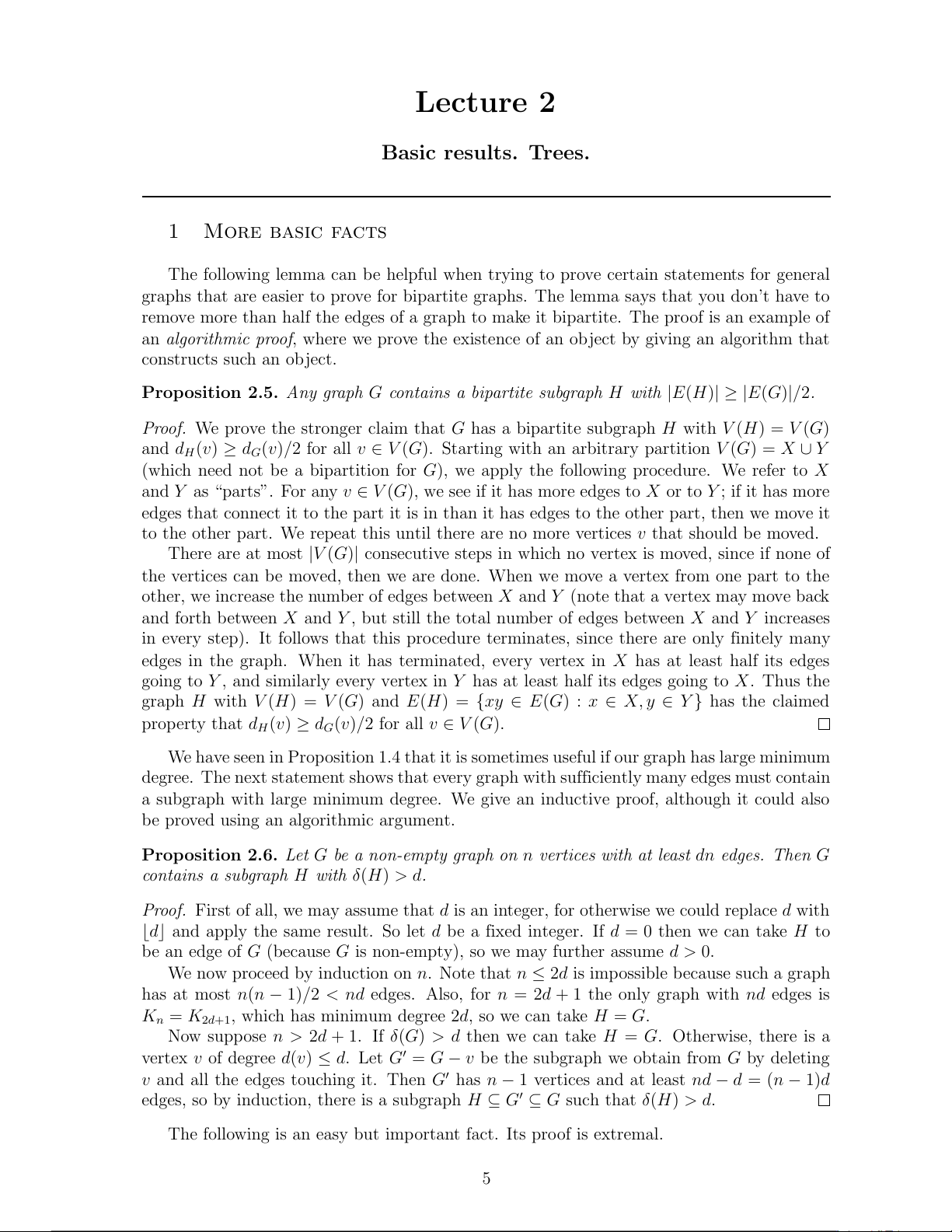
Proposition 2.5. Any graph G contains a bipartite subgraph H with |E(H)| ≥ |E(G)|/2.
Proof. We prove the stronger claim that G has a bipartite subgraph H with V (H) = V (G)
and dH(v) ≥ dG(v)/2 for all v ∈ V (G). Starting with an arbitrary partition V (G) = X ∪ Y
(which need not be a bipartition for G), we apply the following procedure. We refer to X
and Y as “parts”. For any v ∈ V (G), we see if it has more edges to X or to Y ; if it has more
edges that connect it to the part it is in than it has edges to the other part, then we move it
to the other part. We repeat this until there are no more vertices v that should be moved.
There are at most |V (G)| consecutive steps in which no vertex is moved, since if none of
the vertices can be moved, then we are done. When we move a vertex from one part to the
other, we increase the number of edges between X and Y (note that a vertex may move back
and forth between X and Y , but still the total number of edges between X and Y increases
in every step). It follows that this procedure terminates, since there are only finitely many
edges in the graph. When it has terminated, every vertex in X has at least half its edges
going to Y , and similarly every vertex in Y has at least half its edges going to X. Thus the
graph H with V (H) = V (G) and E(H) = {xy ∈ E(G) : x ∈ X, y ∈ Y } has the claimed
property that dH(v) ≥ dG(v)/2 for all v ∈ V (G).
We have seen in Proposition 1.4 that it is sometimes useful if our graph has large minimum
degree. The next statement shows that every graph with sufficiently many edges must contain
a subgraph with large minimum degree. We give an inductive proof, although it could also
be proved using an algorithmic argument.
Proposition 2.6. Let G be a non-empty graph on n vertices with at least dn edges. Then G
contains a subgraph H with δ(H) > d.
Proof. First of all, we may assume that d is an integer, for otherwise we could replace d with
bdc and apply the same result. So let d be a fixed integer. If d = 0 then we can take H to
be an edge of G (because G is non-empty), so we may further assume d > 0.
We now proceed by induction on n. Note that n ≤ 2d is impossible because such a graph
has at most n(n − 1)/2 < nd edges. Also, for n = 2d + 1 the only graph with nd edges is
Kn = K2d+1, which has minimum degree 2d, so we can take H = G.
Now suppose n > 2d + 1. If δ(G) > d then we can take H = G. Otherwise, there is a
vertex v of degree d(v) ≤ d. Let G0 = G − v be the subgraph we obtain from G by deleting
v and all the edges touching it. Then G0 has n − 1 vertices and at least nd − d = (n − 1)d
edges, so by induction, there is a subgraph H ⊆ G0 ⊆ G such that δ(H) > d.
The following is an easy but important fact. Its proof is extremal. 5
Proposition 2.7. Every u-v walk W contains a u-v path.
Proof. Let v1v2 . . . vk be a shortest u-v walk in W (more precisely, in the graph defined by
the edges of W ), so u = v1 and v = vk. We claim that this walk is in fact a path. Indeed,
if vi = vj for some i < j, then v1v2 . . . vivj+1 . . . vk is also a u-v walk, and it is shorter (has
fewer edges), which is not possible. So the shortest walk has no repeated vertices, i.e., it is a path.
This fact has the useful corollaries that we can replace paths with walks in some of our definitions:
• The distance d(u, v) is equal to the length of the shortest u-v walk.
• A graph is connected if and only if every pair of vertices u, v is connected by a walk.
The latter connectivity property is sometimes easier to check. Also, it clearly implies that
connectivity is an equivalence relation.
Our last basic result gives a connection between the number of edges and the number of
connected components in a graph.
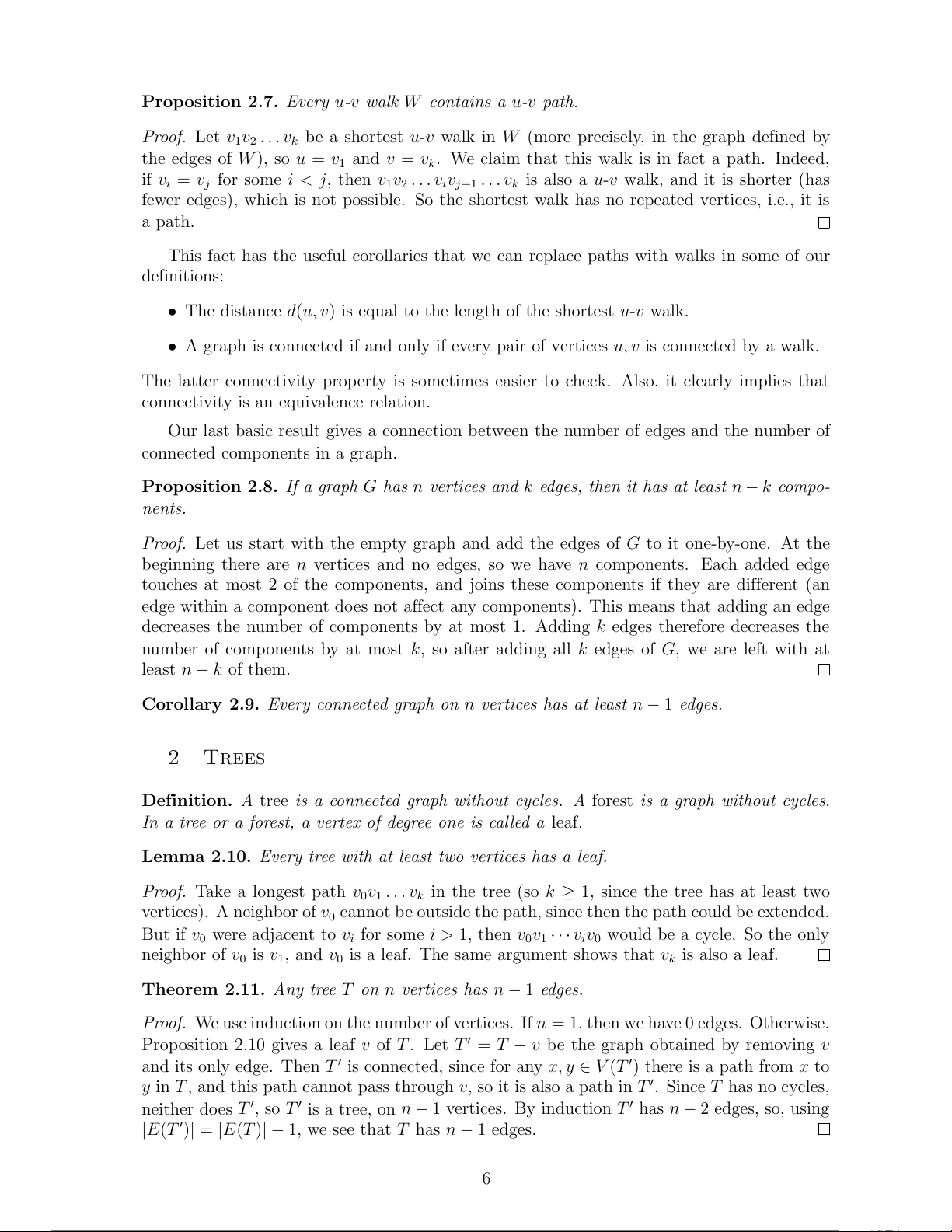
Proposition 2.8. If a graph G has n vertices and k edges, then it has at least n − k compo- nents.
Proof. Let us start with the empty graph and add the edges of G to it one-by-one. At the
beginning there are n vertices and no edges, so we have n components. Each added edge
touches at most 2 of the components, and joins these components if they are different (an
edge within a component does not affect any components). This means that adding an edge
decreases the number of components by at most 1. Adding k edges therefore decreases the
number of components by at most k, so after adding all k edges of G, we are left with at least n − k of them.
Corollary 2.9. Every connected graph on n vertices has at least n − 1 edges. 2 Trees
Definition. A tree is a connected graph without cycles. A forest is a graph without cycles.
In a tree or a forest, a vertex of degree one is called a leaf.
Lemma 2.10. Every tree with at least two vertices has a leaf.
Proof. Take a longest path v0v1 . . . vk in the tree (so k ≥ 1, since the tree has at least two
vertices). A neighbor of v0 cannot be outside the path, since then the path could be extended.
But if v0 were adjacent to vi for some i > 1, then v0v1 · · · viv0 would be a cycle. So the only
neighbor of v0 is v1, and v0 is a leaf. The same argument shows that vk is also a leaf.
Theorem 2.11. Any tree T on n vertices has n − 1 edges.
Proof. We use induction on the number of vertices. If n = 1, then we have 0 edges. Otherwise,
Proposition 2.10 gives a leaf v of T . Let T 0 = T − v be the graph obtained by removing v
and its only edge. Then T 0 is connected, since for any x, y ∈ V (T 0) there is a path from x to
y in T , and this path cannot pass through v, so it is also a path in T 0. Since T has no cycles,
neither does T 0, so T 0 is a tree, on n − 1 vertices. By induction T 0 has n − 2 edges, so, using
|E(T 0)| = |E(T )| − 1, we see that T has n − 1 edges. 6
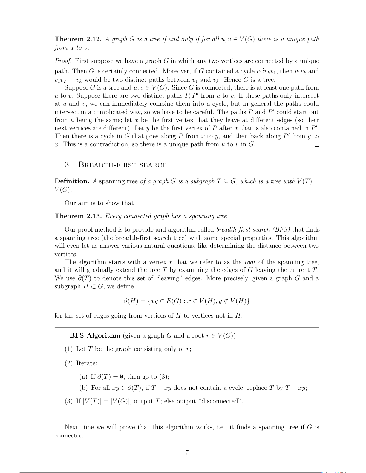
Theorem 2.12. A graph G is a tree if and only if for all u, v ∈ V (G) there is a unique path from u to v.
Proof. First suppose we have a graph G in which any two vertices are connected by a unique .
path. Then G is certainly connected. Moreover, if G contained a cycle v . 1.vkv1, then v1vk and
v1v2 · · · vk would be two distinct paths between v1 and vk. Hence G is a tree.
Suppose G is a tree and u, v ∈ V (G). Since G is connected, there is at least one path from
u to v. Suppose there are two distinct paths P, P 0 from u to v. If these paths only intersect
at u and v, we can immediately combine them into a cycle, but in general the paths could
intersect in a complicated way, so we have to be careful. The paths P and P 0 could start out
from u being the same; let x be the first vertex that they leave at different edges (so their
next vertices are different). Let y be the first vertex of P after x that is also contained in P 0.
Then there is a cycle in G that goes along P from x to y, and then back along P 0 from y to
x. This is a contradiction, so there is a unique path from u to v in G. 3 Breadth-first search
Definition. A spanning tree of a graph G is a subgraph T ⊆ G, which is a tree with V (T ) = V (G). Our aim is to show that
Theorem 2.13. Every connected graph has a spanning tree.
Our proof method is to provide and algorithm called breadth-first search (BFS) that finds
a spanning tree (the breadth-first search tree) with some special properties. This algorithm
will even let us answer various natural questions, like determining the distance between two vertices.
The algorithm starts with a vertex r that we refer to as the root of the spanning tree,
and it will gradually extend the tree T by examining the edges of G leaving the current T .
We use ∂(T ) to denote this set of “leaving” edges. More precisely, given a graph G and a subgraph H ⊂ G, we define
∂(H) = {xy ∈ E(G) : x ∈ V (H), y 6∈ V (H)}
for the set of edges going from vertices of H to vertices not in H.
BFS Algorithm (given a graph G and a root r ∈ V (G))
(1) Let T be the graph consisting only of r; (2) Iterate:
(a) If ∂(T ) = ∅, then go to (3);
(b) For all xy ∈ ∂(T ), if T + xy does not contain a cycle, replace T by T + xy;
(3) If |V (T )| = |V (G)|, output T ; else output “disconnected”.
Next time we will prove that this algorithm works, i.e., it finds a spanning tree if G is connected. 7 Lecture 3
BFS. Euler tours. Hamilton cycles. 1 Breadth-first search
As it turns out, BFS not only finds a spanning tree of G, but it finds a shortest path from its root to any other vertex.
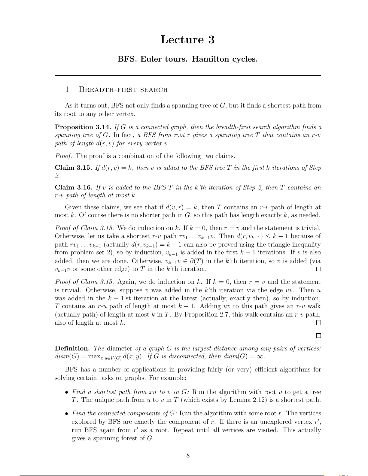
Proposition 3.14. If G is a connected graph, then the breadth-first search algorithm finds a
spanning tree of G. In fact, a BFS from root r gives a spanning tree T that contains an r-v
path of length d(r, v) for every vertex v.
Proof. The proof is a combination of the following two claims.
Claim 3.15. If d(r, v) = k, then v is added to the BFS tree T in the first k iterations of Step 2
Claim 3.16. If v is added to the BFS T in the k’th iteration of Step 2, then T contains an r-v path of length at most k.
Given these claims, we see that if d(v, r) = k, then T contains an r-v path of length at
most k. Of course there is no shorter path in G, so this path has length exactly k, as needed.
Proof of Claim 3.15. We do induction on k. If k = 0, then r = v and the statement is trivial.
Otherwise, let us take a shortest r-v path rv1 . . . vk (
−1v. Then d r, vk−1) ≤ k − 1 because of
path rv1 . . . vk−1 (actually d(r, vk−1) = k − 1 can also be proved using the triangle-inequality
from problem set 2), so by induction, vk is added in the first 1 iterations. If is also −1 k − v
added, then we are done. Otherwise, vk ) in the is added (via −1v ∈ ∂(T k’th iteration, so v
vk−1v or some other edge) to T in the k’th iteration.
Proof of Claim 3.15. Again, we do induction on k. If k = 0, then r = v and the statement
is trivial. Otherwise, suppose v was added in the k’th iteration via the edge uv. Then u
was added in the k − 1’st iteration at the latest (actually, exactly then), so by induction,
T contains an r-u path of length at most k − 1. Adding uv to this path gives an r-v walk
(actually path) of length at most k in T . By Proposition 2.7, this walk contains an r-v path, also of length at most k.
Definition. The diameter of a graph G is the largest distance among any pairs of vertices: diam(G) = maxx,y )
∈V (G) d(x, y . If G is disconnected, then diam(G) = ∞.
BFS has a number of applications in providing fairly (or very) efficient algorithms for
solving certain tasks on graphs. For example:
• Find a shortest path from xu to v in G: Run the algorithm with root u to get a tree
T . The unique path from u to v in T (which exists by Lemma 2.12) is a shortest path.
• Find the connected components of G: Run the algorithm with some root r. The vertices
explored by BFS are exactly the component of r. If there is an unexplored vertex r0,
run BFS again from r0 as a root. Repeat until all vertices are visited. This actually gives a spanning forest of G. 8
• Compute diam(G): For each pair of vertices, we can find a shortest path and thus the
distance. Do this for all pairs and take the largest distance.
• Find a shortest cycle in G: For every edge uv, find a shortest path between u and v
in G − uv (if it exists), then combine this path with uv to get a cycle. (This will be a
shortest cycle through uv.) Compare all these cycles to find the shortest.
• Determine if G is bipartite: Determine the connected components of G. In every
component H, select a root r, and partition the vertices into X = {x ∈ V (H) :
d(r, x) is even} and Y = {y ∈ V (H) : d(r, y) is odd}. Then H is bipartite if and only
if X and Y have no internal edges (see the proof of Theorem 1.2), and G is bipartite if
and only if every component is bipartite.
Not all of these algorithms are the most efficient, but they are already much better than
brute force approaches that go over all possible answers. There are all kinds of algorithms
that do these tasks faster, but in this course, we don’t care too much about efficiency, and
we focus on the graph-theoretical aspects (in particular, proving that the algorithms work).
We should emphasize, though, that for finding shortest paths between two vertices, BFS
is the best general algorithm. For example, Dijkstra’s algorithm, a variant of BFS that works
for graphs with positive edge weights (representing, e.g, the lengths of streets) is directly used by routing softwares. 2 Euler tours
Definition. A trail is a walk with no repeated edges. A tour is a closed trail (i.e., one that
starts and ends at the same vertex).
Definition. An Euler (or Eulerian) trail in a (multi)graph G = (V, E) is a trail in G passing
through every edge (exactly once). An Euler tour is a tour in G passing through every edge.
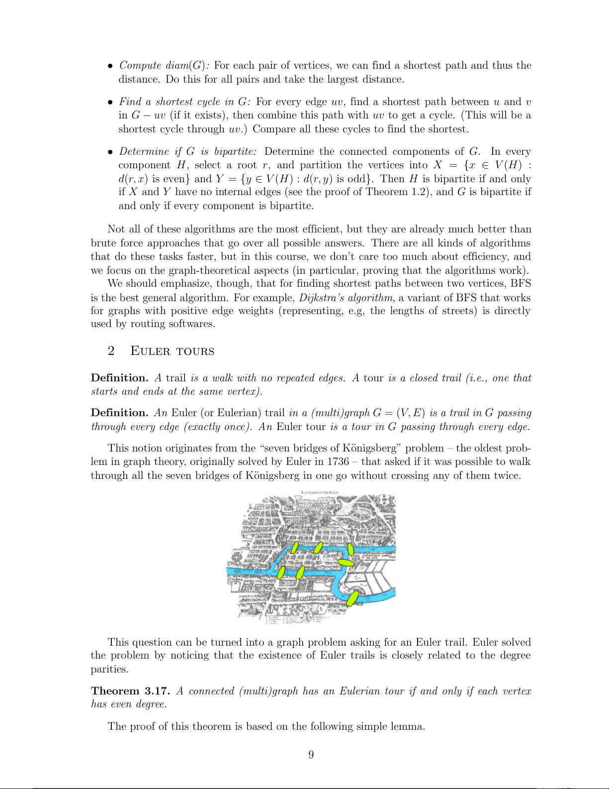
This notion originates from the “seven bridges of K¨onigsberg” problem – the oldest prob-
lem in graph theory, originally solved by Euler in 1736 – that asked if it was possible to walk
through all the seven bridges of K¨onigsberg in one go without crossing any of them twice.
This question can be turned into a graph problem asking for an Euler trail. Euler solved
the problem by noticing that the existence of Euler trails is closely related to the degree parities.
Theorem 3.17. A connected (multi)graph has an Eulerian tour if and only if each vertex has even degree.
The proof of this theorem is based on the following simple lemma. 9
Lemma 3.18. In a graph where all vertices have even degree, every maximal trail is a closed trail.
Proof. Let T be a maximal trail. If T is not closed, then T has an odd number of edges
incident to the final vertex v. However, as v has even degree, there is an edge touching v
that is not contained in T . This edge can be used to extend T to a longer trail, contradicting the maximality of T .
Proof of Theorem 3.17. To see that the condition is necessary, suppose G has an Eulerian
tour C. If a vertex v was visited k times in the tour C, then each visit used 2 edges incident
to v (one incoming edge and one outgoing edge). Thus, d(v) = 2k, which is even.
To see that the condition is sufficient, let G be a connected graph with even degrees. Let
T = e1e2 . . . e` (where ei = (vi−1, vi)) be a longest trail in G. Then it is maximal, of course.
According to the Lemma, T is closed, i.e., v0 = v`. G is connected, so if T does not include
all the edges of G then there is an edge e outside of T that touches it, i.e., e = uvi for some
vertex vi in T . Since T is closed, we can start walking through it at any vertex. But if we
start at vi then we can append the edge e at the end: T 0 = ei+1 . . . e`e1e2 . . . eie is a trail in
G which is longer than T , contradicting the fact that T is a longest trail in G. Thus, T must
include all the edges of G and so it is an Eulerian tour.
Corollary 3.19. A connected multigraph G has an Euler trail if and only if it has either 0 or 2 vertices of odd degree.
Proof. Suppose T is an Euler trail from vertex u to vertex v. If u = v then T is an Eulerian
tour and so by Theorem 3.17, it follows that all the vertices in G have even degree. If u 6= v
then let us add a new edge e = uv to G. In this new multigraph G ∪ {e}, T ∪ {e} is an Euler
tour. By Theorem 3.17 we see that all the degrees in G ∪ {e} are even. This means that in
the original multigraph G, the vertices u, v are the only ones that have odd degree.
Now we prove the other direction of the corollary. If G has no vertices of odd degree then
by Theorem 3.17 it contains an Eulerian tour which is also an Eulerian trail. Suppose now
that G has 2 vertices u, v of odd degree. Then add a new edge e to G. Now all vertices of
the resulting multigraph G ∪ {e} have even degree, so, by Theorem 3.17, it has an Eulerian
tour C. Removing the edge e from C gives an Eulerian trail of G from u to v. 3 Hamilton cycles
Euler trails are walks that use each edge exactly once. But what if we want to use each vertex exactly once?
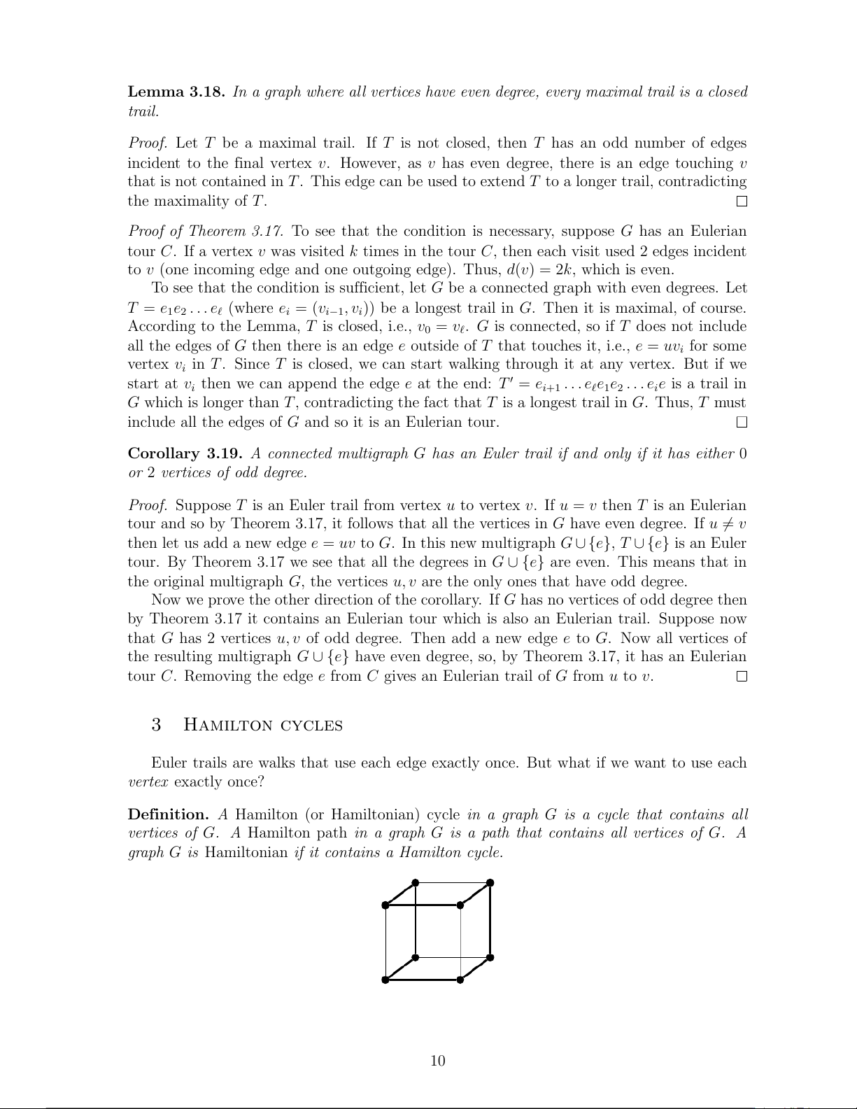
Definition. A Hamilton (or Hamiltonian) cycle in a graph G is a cycle that contains all
vertices of G. A Hamilton path in a graph G is a path that contains all vertices of G. A
graph G is Hamiltonian if it contains a Hamilton cycle. 10
Although the proof of Theorem 3.17 is not really described in an algorithmic way, it can
actually be turned into an efficient algorithm. However, no good algorithm is known that
would find a Hamilton cycle in a graph: nothing that would be much better a brute-force
algorithm that tries every possible way to visit all vertices in the graph. Deciding if G is
Hamiltonian is a so-called NP-hard (actually, NP-complete) problem. Loosely speaking, this
means that an efficient algorithm for this problem could be transformed into an efficient
algorithm for many other problems that are also considered algorithmically difficult.
Definition. The girth of a graph G is the length of the shortest cycle contained in G. The
circumference is the length of the longest cycle contained in G.
For example, the complete graph Kn for n ≥ 3 has girth 3 and circumference n.
We have seen that computing the girth of a graph can be done fairly efficiently using BFS.
But finding the circumference is even more difficult than deciding if a graph is Hamiltonian
(because a graph has a Hamilton cycle if and only if its circumference is n).
Another related problem is to find a shortest Hamilton cycle in a graph with weighted
edges; this is called the travelling salesman problem (TSP) and is one of the most famous
computationally hard problems, with many real-life applications.
Although we have no general algorithm or recipe for finding Hamilton cycles, we can still
prove some theorems that are useful in certain situations. Our first example is a necessary condition for Hamiltonicity.
Given a graph G and a set S ⊂ V (G) of vertices, we write G − S for the graph obtained
by removing the vertices of S from G, along with all the edges touching the vertices in S.
Lemma 3.20. If G has a Hamilton cycle, then for all S ⊂ V (G), G − S has at most |S| connected components.
Proof. The Hamilton cycle must visit all the components of G − S (viewed as subgraphs of
G), and to get from one component to another the cycle must pass through a vertex of S.
Thus every component is connected to S by two edges of the cycle (and possibly by other
edges not in the cycle). Since every vertex is incident to two edges of the cycle, we have that
twice the number of components is at most twice the number of vertices of S.
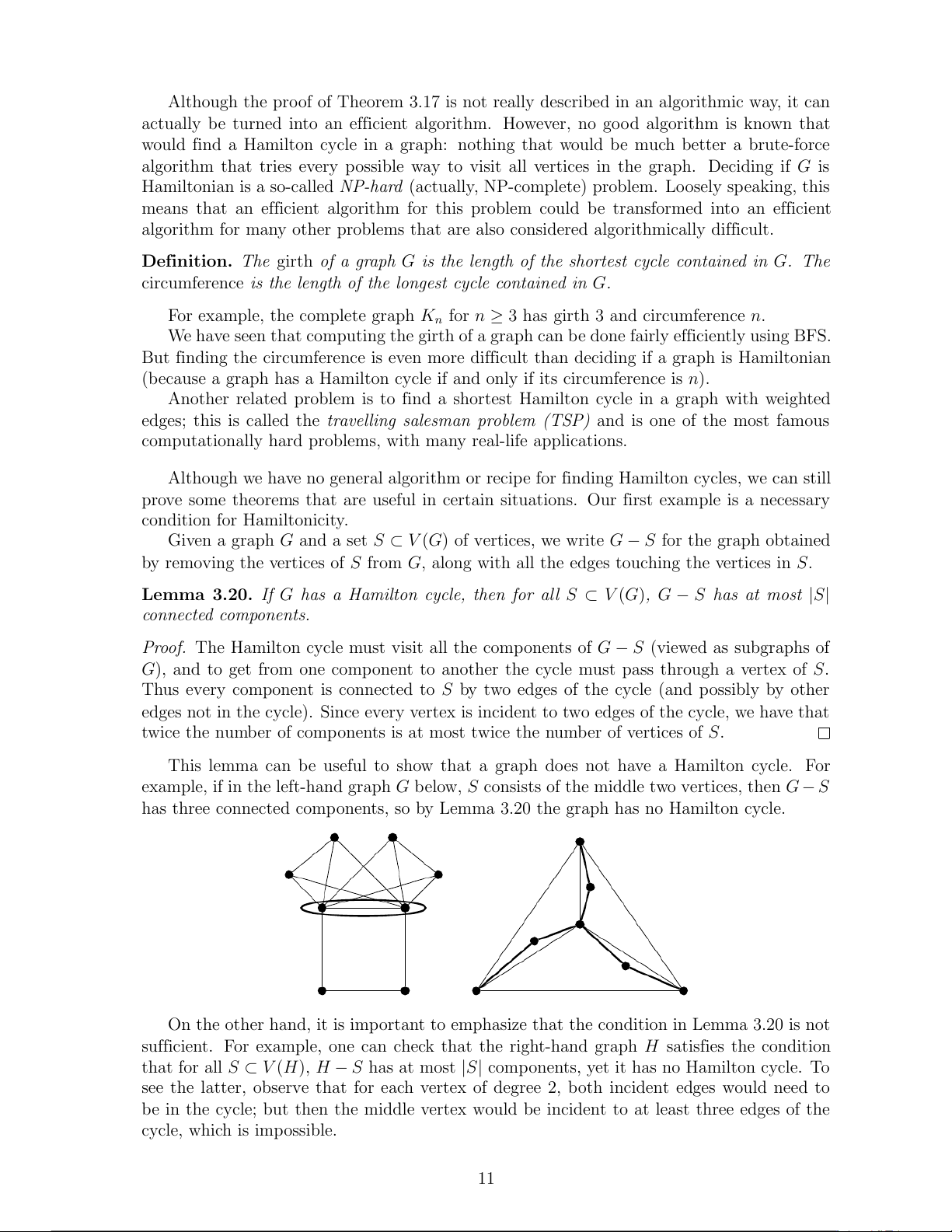
This lemma can be useful to show that a graph does not have a Hamilton cycle. For
example, if in the left-hand graph G below, S consists of the middle two vertices, then G − S
has three connected components, so by Lemma 3.20 the graph has no Hamilton cycle.
On the other hand, it is important to emphasize that the condition in Lemma 3.20 is not
sufficient. For example, one can check that the right-hand graph H satisfies the condition
that for all S ⊂ V (H), H − S has at most |S| components, yet it has no Hamilton cycle. To
see the latter, observe that for each vertex of degree 2, both incident edges would need to
be in the cycle; but then the middle vertex would be incident to at least three edges of the cycle, which is impossible. 11 Lecture 4 Hamilton cycles. 1
Sufficient conditions for Hamiltonicity
First, we will show that a graph with many edges must have a Hamilton cycle. Unfor-
tunately, there is no chance to get a very good bound on the number of edges sufficient
to guarantee a Hamilton cycle, because there are “almost complete” graphs that are not Hamiltonian.
Take for instance the graph G consisting of Kn
and an additional vertex connected to −1 a single vertex of K
n−1. This graph has n−1 + 1 edges (so only misses n − 2 edges), but it is 2
not Hamiltonian, because it has a vertex of degree 1. Our next result shows that any graph
with more edges contains a Hamilton cycle.
Theorem 4.21. If G is an n-vertex graph with |E(G)| > n−1 + 1 edges, then G contains a 2 Hamilton cycle.
Proof. We apply induction on n. The statement is clearly true for n = 1, 2, 3, so we assume n > 3.
We claim that G has a vertex v of degree at least n − 2. Indeed, otherwise every vertex has degree at most n − 3, so P d(v) n(n − 3) (n − 1)(n − 2) n − 1 |E(G)| = v ≤ < = , 2 2 2 2 contradicting our assumption.
Now let G0 = G − v, so G0 has n − 1 vertices. We distinguish the two cases d(v) = n − 2 and d(v) = n − 1. Suppose d(v) = n − 2. Then n − 1 n − 2
|E(G0)| = |E(G)| − (n − 2) > + 1 − (n − 2) = + 1, 2 2
so G0 has a Hamilton cycle C by induction. Since d(v) = n −2 and n > 3, v must be adjacent
to two consecutive vertices of this cycle, x and y. Then we can remove the edge xy from C
and replace it by xv and vy to get a Hamilton cycle in G.
Now suppose d(v) = n − 1. In this case we only have |E(G0)| > n−2, so we cannot apply 2
induction right away. If G0 is complete, then G0 has a Hamilton cycle, and we can add v as
in the previous case (in fact, as d(v) = n − 1, v is now adjacent to every vertex of the cycle).
Otherwise, there is an edge xy missing from G0. Let us look at the graph G0 + xy that
we get by adding xy to G0. Now this graph has more than n−2 + 1 edges, so we can apply 2
induction to find a Hamilton cycle C in it. If C does not contain xy, then we can again add
v as in the previous case. If C does contain xy, then replacing xy with the path xvy in C gives a Hamilton cycle in G.
As mentioned before, the condition in the theorem above is somewhat weak in the sense
that many graphs that have a Hamilton cycle do not satisfy the condition. The following
sufficient condition does better by looking at the minimum degree instead of the total number
of edges. Note that we have previously seen that every graph G has a cycle of length at least
δ(G)+1. The following theorem says that something much stronger is true when the minimum degree is at least |V (G)|/2. 12
Theorem 4.22 (Dirac). Let G be a graph on n ≥ 3 vertices. If δ(G) ≥ n, then G contains 2 a Hamilton cycle.
Proof. First observe that G must be connected, because each component contains at least
δ(G) + 1 > n/2 vertices, so G cannot have more than one components.
Take a longest path P = v1v2 . . . vk in G. By maximality, all neighbors of v1 and vk are
in the path. Let us say that an edge vivi+1 is type-1 if vi+1 ∈ N(v1), and let us say that it
is type-2 if vi ∈ N(vk). As δ(G) ≥ n/2, we have at least n/2 type-1 and n/2 type-2 edges
in P . But P has at most n − 1 edges, so some edge vjvj+1 is both type-1 and type-2, i.e.,
v1vj+1 and vjvk are edges of G. Then C = P − vjvj+1 + v1vj+1 + vjvk = vj . . . v1vj+1 . . . vkvi is a cycle.
In fact, C is a Hamilton cycle. Indeed, suppose not all vertices are contained in C. Since
G is connected, there must be an edge uvi where u /
∈ C. Then there is a path that goes from
u to vi and then all around the cycle C to a neighbor of vi. This path contains k + 1 vertices,
contradicting the maximality of P .
This theorem is again best possible, in the sense that a weaker bound on the minimum
degree would not imply a Hamilton cycle. Take for instance the graph G consisting of two
copies of Kk sharing a single vertex. This graph has n = 2k − 1 vertices and minimum degree
δ(G) = k − 1 = n−1, but no Hamilton cycle, because deleting the shared vertex creates two 2
components, contradicting Lemma 3.20.
It is easy to check that the proof of Dirac’s theorem works for the following strengthening, as well:
Theorem 4.23 (Ore). Let G be a graph on n ≥ 3 vertices. If d(u) + d(v) ≥ n for any
non-adjacent vertices u and v, then G contains a Hamilton cycle.
Using this theorem, one can also obtain a short proof of Theorem 4.21 (see problem set),
so one can think of Ore’s theorem as a common generalization of Theorems 4.21 and 4.22.
We will give one more sufficient condition, that is not a corollary of Ore’s theorem. We need the following definition.
Definition. Let G be a graph. A vertex set I ⊆ V (G) is called independent in G if no two
vertices of I are connected by an edge of G. The independence number α(G) is the size of
the largest independent set in G.
For example, α(Kn) = 1, α(Kn,m) = max(n, m), and the independence number of the
empty graph on n vertices is n.
Theorem 4.24. Let G be a graph on n ≥ 3 vertices. If G has at least α(G) vertices of degree
n − 1, then it contains a Hamilton cycle.
Proof. Let k = α(G), and let us take a longest cycle C in G. We will prove that C is a
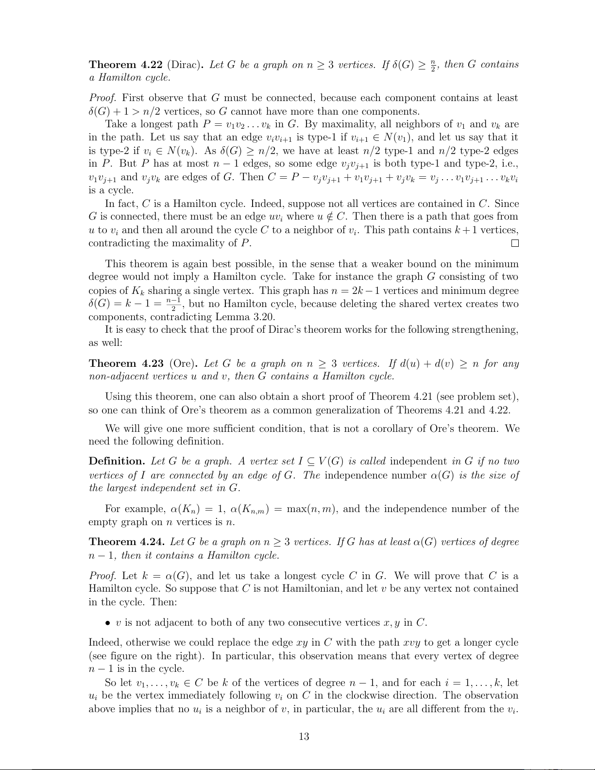
Hamilton cycle. So suppose that C is not Hamiltonian, and let v be any vertex not contained in the cycle. Then:
• v is not adjacent to both of any two consecutive vertices x, y in C.
Indeed, otherwise we could replace the edge xy in C with the path xvy to get a longer cycle
(see figure on the right). In particular, this observation means that every vertex of degree n − 1 is in the cycle.
So let v1, . . . , vk ∈ C be k of the vertices of degree n − 1, and for each i = 1, . . . , k, let
ui be the vertex immediately following vi on C in the clockwise direction. The observation
above implies that no ui is a neighbor of v, in particular, the ui are all different from the vi. 13
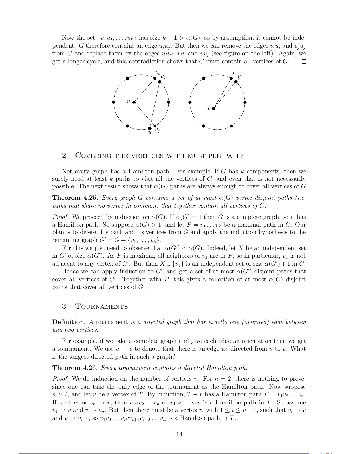
Now the set {v, u1, . . . , uk} has size k + 1 > α(G), so by assumption, it cannot be inde-
pendent. G therefore contains an edge uiuj. But then we can remove the edges viui and vjuj
from C and replace them by the edges uiuj, viv and vvj (see figure on the left). Again, we
get a longer cycle, and this contradiction shows that C must contain all vertices of G. vi x ui y v v u vj j 2
Covering the vertices with multiple paths
Not every graph has a Hamilton path. For example, if G has k components, then we
surely need at least k paths to visit all the vertices of G, and even that is not necessarily
possible. The next result shows that α(G) paths are always enough to cover all vertices of G
Theorem 4.25. Every graph G contains a set of at most α(G) vertex-disjoint paths (i.e.
paths that share no vertex in common) that together contain all vertices of G.
Proof. We proceed by induction on α(G). If α(G) = 1 then G is a complete graph, so it has
a Hamilton path. So suppose α(G) > 1, and let P = v1 . . . vk be a maximal path in G. Our
plan is to delete this path and its vertices from G and apply the induction hypothesis to the
remaining graph G0 = G − {v1, . . . , vk}.
For this we just need to observe that α(G0) < α(G). Indeed, let X be an independent set
in G0 of size α(G0). As P is maximal, all neighbors of v1 are in P , so in particular, v1 is not
adjacent to any vertex of G0. But then X ∪ {v1} is an independent set of size α(G0) + 1 in G.
Hence we can apply induction to G0, and get a set of at most α(G0) disjoint paths that
cover all vertices of G0. Together with P , this gives a collection of at most α(G) disjoint
paths that cover all vertices of G. 3 Tournaments
Definition. A tournament is a directed graph that has exactly one (oriented) edge between any two vertices.
For example, if we take a complete graph and give each edge an orientation then we get
a tournament. We use u → v to denote that there is an edge uv directed from u to v. What
is the longest directed path in such a graph?
Theorem 4.26. Every tournament contains a directed Hamilton path.
Proof. We do induction on the number of vertices n. For n = 2, there is nothing to prove,
since one can take the only edge of the tournament as the Hamilton path. Now suppose
n > 2, and let v be a vertex of T . By induction, T − v has a Hamilton path P = v1v2 . . . vn.
If v → v1 or vn → v, then vv1v2 . . . vn or v1v2 . . . vnv is a Hamilton path in T . So assume
v1 → v and v → vn. But then there must be a vertex vi with 1 ≤ i ≤ n − 1, such that vi → v
and v → vi+1, so v1v2 . . . vivvi+1vi+2 . . . vn is a Hamilton path in T . 14
Of course, not every tournament contains a directed Hamilton cycle. In fact, there is a
tournament that does not contain any cycle, whatsoever: the so-called transitive tournament
on vertex set {1, . . . , n} where each edge is oriented from the smaller endpoint to the larger
one. But can we find conditions for the existence of a Hamilton cycle?
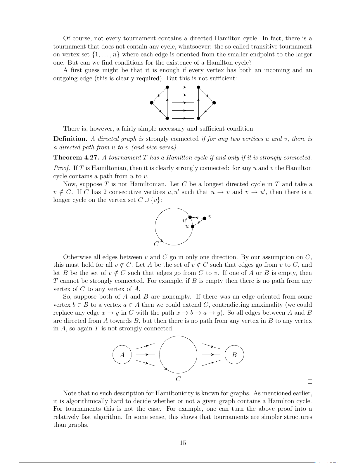
A first guess might be that it is enough if every vertex has both an incoming and an
outgoing edge (this is clearly required). But this is not sufficient:
There is, however, a fairly simple necessary and sufficient condition.
Definition. A directed graph is strongly connected if for any two vertices u and v, there is
a directed path from u to v (and vice versa).
Theorem 4.27. A tournament T has a Hamilton cycle if and only if it is strongly connected.
Proof. If T is Hamiltonian, then it is clearly strongly connected: for any u and v the Hamilton
cycle contains a path from u to v.
Now, suppose T is not Hamiltonian. Let C be a longest directed cycle in T and take a v /
∈ C. If C has 2 consecutive vertices u, u0 such that u → v and v → u0, then there is a
longer cycle on the vertex set C ∪ {v}: v u0u C
Otherwise all edges between v and C go in only one direction. By our assumption on C, this must hold for all v / ∈ C. Let A be the set of v /
∈ C such that edges go from v to C, and let B be the set of v /
∈ C such that edges go from C to v. If one of A or B is empty, then
T cannot be strongly connected. For example, if B is empty then there is no path from any
vertex of C to any vertex of A.
So, suppose both of A and B are nonempty. If there was an edge oriented from some
vertex b ∈ B to a vertex a ∈ A then we could extend C, contradicting maximality (we could
replace any edge x → y in C with the path x → b → a → y). So all edges between A and B
are directed from A towards B, but then there is no path from any vertex in B to any vertex
in A, so again T is not strongly connected. A B C
Note that no such description for Hamiltonicity is known for graphs. As mentioned earlier,
it is algorithmically hard to decide whether or not a given graph contains a Hamilton cycle.
For tournaments this is not the case. For example, one can turn the above proof into a
relatively fast algorithm. In some sense, this shows that tournaments are simpler structures than graphs. 15 Lecture 5 Planar graphs. 1 Drawings of graphs
We have so far only considered abstract graphs, although we often used pictures to il-
lustrate the graph. In this lecture, we prove some facts about pictures of graphs and their
properties. To set this on a firm footing, we give a formal definition of what we mean by
“picture”, although in most of the lecture we will be less formal.
Definition. A drawing of a graph G consists of an injective map f : V (G) → R2, and
a curve γxy (the image of an injective continuous map [0, 1] → R2) from x to y for every
xy ∈ E(G), such that f(z) 6∈ γxy for any vertex z 6= x, y. A drawing is planar if the curves
γxy do not intersect each other except possibly at endpoints.
Definition. A graph is planar if it has a planar drawing.
For example, the graphs K4 and K2,3 are planar graphs.
To show that a graph is planar, we only have to supply a planar drawing. It is often a
little harder to show that a graph is not planar.
Proposition 5.28. The graph K5 is not planar.
Proof. The graph contains a K3, which can basically be drawn in only one way. If in a
drawing the fourth vertex is inside this K3 and the fifth is outside, then the edge between
them must cross the K3, which means that the drawing is not planar. If both vertices are
inside the K3, then the three edges of one vertex divide the inside of K3 into three regions.
The other vertex must then be in one of these regions, and one vertex of K3 is outside this
region, so again, the edge between these two vertices crosses the boundary of the region. A
similar argument applies when both vertices are outside the K3.
Note that this proof heavily relied on the fact that an edge connecting a vertex inside of
K3 (or any other cycle) to a vertex outside must cross the K3 (or cycle). This is a highly non-
trivial statement that depends on a strong topological theorem called the Jordan Curve
Theorem, that states that every non-self-intersecting closed curve in R2 divides R2 into an
inside and an outside, and any path between a point inside and a point outside must pass
through the closed curve. We remark that this theorem is specific to the plane: it is not
always true in some other surfaces, for example, on a torus.
The Jordan Curve Theorem is well beyond the scope of this course. To avoid using such
heavy machinery, we could replace continuous curves with polygonal paths in the definition
of drawings, where a polygonal path is a special curve, whose image is a union of finitely
many segments. The Jordan Curve Theorem is much easier to prove for such paths.
Nevertheless, many technicalities arise when adding edges to drawings, even if we use
polygonal paths, but we are going to ignore these for clarity. Therefore, our proofs concern-
ing planarity will sometimes appeal to intuition, hence they will not always be completely rigorous. 16 2 Euler’s formula
One important property that distinguishes planar drawings from general graph drawings
is that plane drawings have faces.
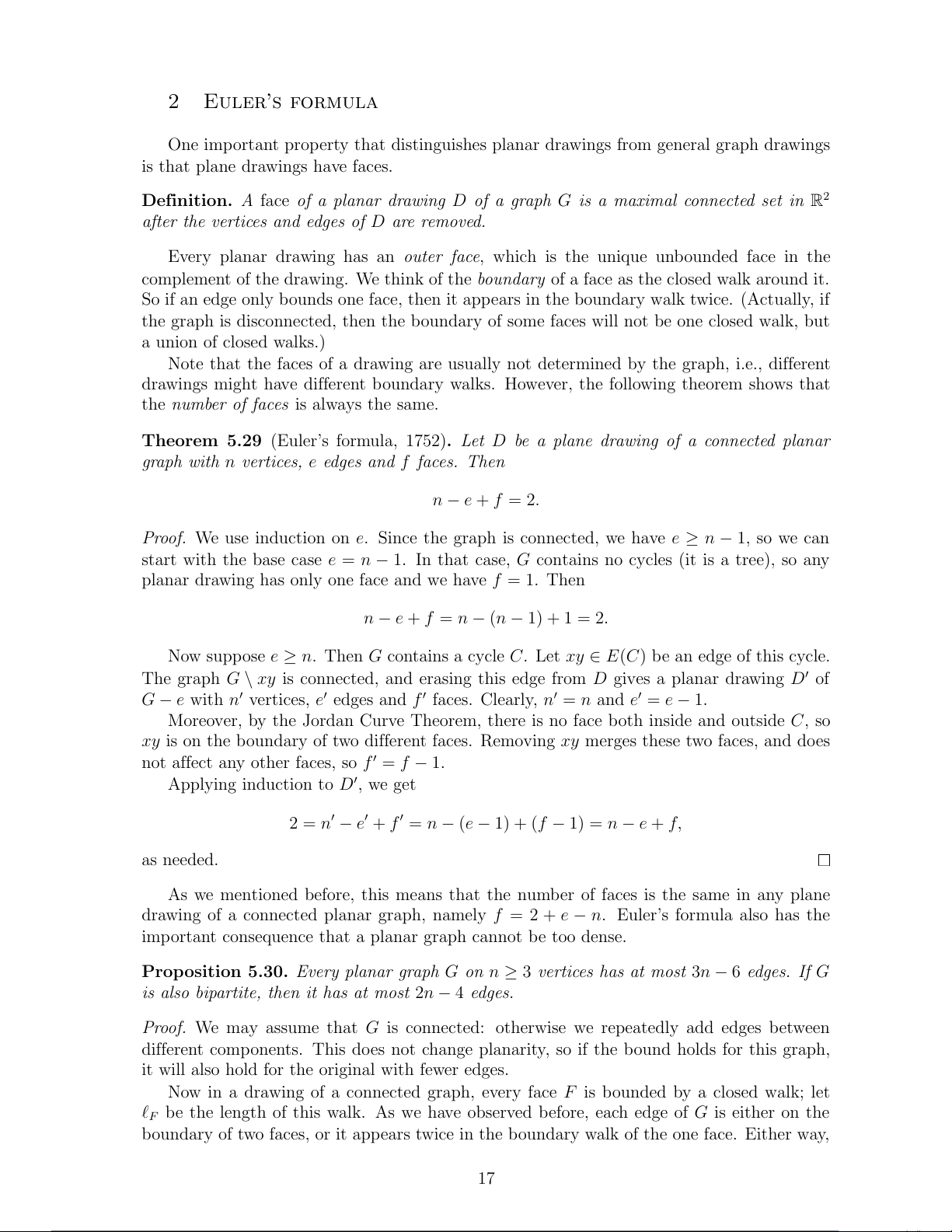
Definition. A face of a planar drawing D of a graph G is a maximal connected set in R2
after the vertices and edges of D are removed.
Every planar drawing has an outer face, which is the unique unbounded face in the
complement of the drawing. We think of the boundary of a face as the closed walk around it.
So if an edge only bounds one face, then it appears in the boundary walk twice. (Actually, if
the graph is disconnected, then the boundary of some faces will not be one closed walk, but a union of closed walks.)
Note that the faces of a drawing are usually not determined by the graph, i.e., different
drawings might have different boundary walks. However, the following theorem shows that
the number of faces is always the same.
Theorem 5.29 (Euler’s formula, 1752). Let D be a plane drawing of a connected planar
graph with n vertices, e edges and f faces. Then n − e + f = 2.
Proof. We use induction on e. Since the graph is connected, we have e ≥ n − 1, so we can
start with the base case e = n − 1. In that case, G contains no cycles (it is a tree), so any
planar drawing has only one face and we have f = 1. Then
n − e + f = n − (n − 1) + 1 = 2.
Now suppose e ≥ n. Then G contains a cycle C. Let xy ∈ E(C) be an edge of this cycle.
The graph G \ xy is connected, and erasing this edge from D gives a planar drawing D0 of
G − e with n0 vertices, e0 edges and f0 faces. Clearly, n0 = n and e0 = e − 1.
Moreover, by the Jordan Curve Theorem, there is no face both inside and outside C, so
xy is on the boundary of two different faces. Removing xy merges these two faces, and does
not affect any other faces, so f 0 = f − 1.
Applying induction to D0, we get
2 = n0 − e0 + f0 = n − (e − 1) + (f − 1) = n − e + f, as needed.
As we mentioned before, this means that the number of faces is the same in any plane
drawing of a connected planar graph, namely f = 2 + e − n. Euler’s formula also has the
important consequence that a planar graph cannot be too dense.
Proposition 5.30. Every planar graph G on n ≥ 3 vertices has at most 3n − 6 edges. If G
is also bipartite, then it has at most 2n − 4 edges.
Proof. We may assume that G is connected: otherwise we repeatedly add edges between
different components. This does not change planarity, so if the bound holds for this graph,
it will also hold for the original with fewer edges.
Now in a drawing of a connected graph, every face F is bounded by a closed walk; let
`F be the length of this walk. As we have observed before, each edge of G is either on the
boundary of two faces, or it appears twice in the boundary walk of the one face. Either way, 17
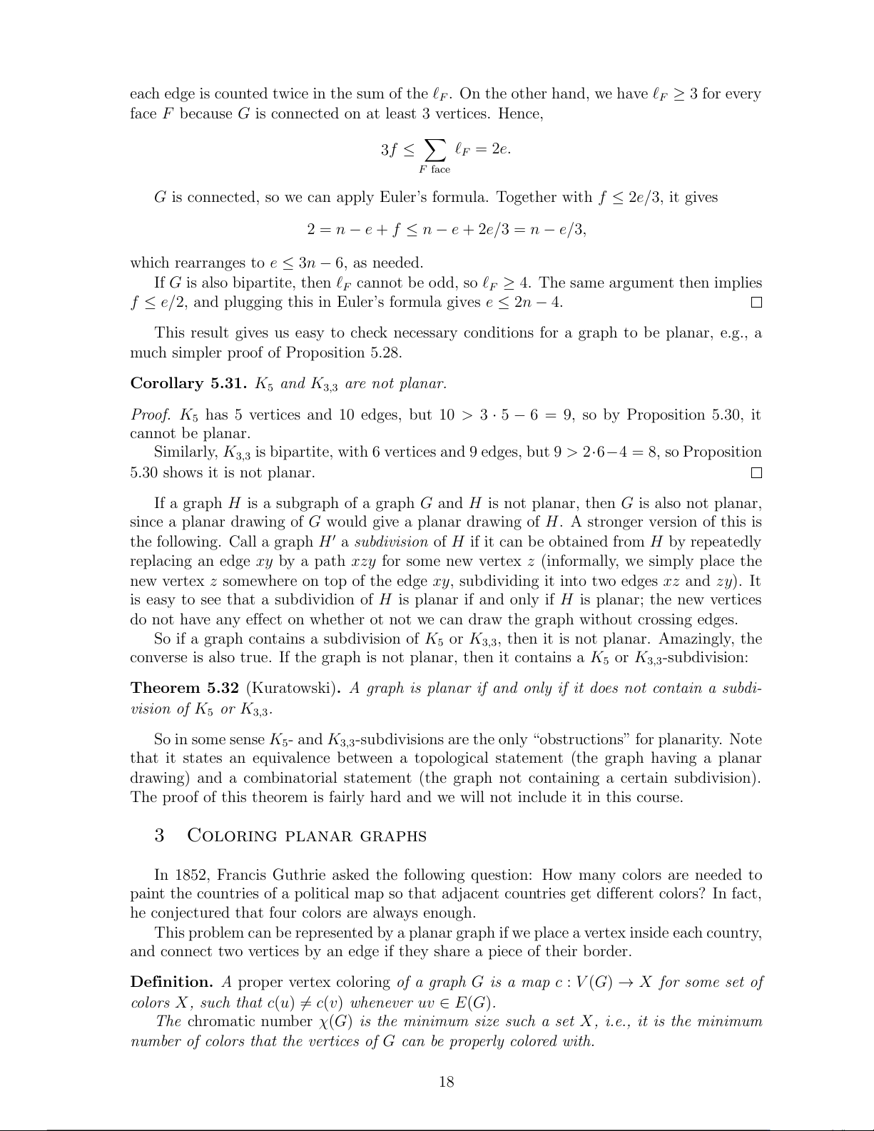
each edge is counted twice in the sum of the `F . On the other hand, we have `F ≥ 3 for every
face F because G is connected on at least 3 vertices. Hence, 3f ≤ X `F = 2e. F face
G is connected, so we can apply Euler’s formula. Together with f ≤ 2e/3, it gives
2 = n − e + f ≤ n − e + 2e/3 = n − e/3,
which rearranges to e ≤ 3n − 6, as needed.
If G is also bipartite, then `F cannot be odd, so `F ≥ 4. The same argument then implies
f ≤ e/2, and plugging this in Euler’s formula gives e ≤ 2n − 4.
This result gives us easy to check necessary conditions for a graph to be planar, e.g., a
much simpler proof of Proposition 5.28.
Corollary 5.31. K5 and K3,3 are not planar.
Proof. K5 has 5 vertices and 10 edges, but 10 > 3 · 5 − 6 = 9, so by Proposition 5.30, it cannot be planar.
Similarly, K3,3 is bipartite, with 6 vertices and 9 edges, but 9 > 2·6−4 = 8, so Proposition 5.30 shows it is not planar.
If a graph H is a subgraph of a graph G and H is not planar, then G is also not planar,
since a planar drawing of G would give a planar drawing of H. A stronger version of this is
the following. Call a graph H0 a subdivision of H if it can be obtained from H by repeatedly
replacing an edge xy by a path xzy for some new vertex z (informally, we simply place the
new vertex z somewhere on top of the edge xy, subdividing it into two edges xz and zy). It
is easy to see that a subdividion of H is planar if and only if H is planar; the new vertices
do not have any effect on whether ot not we can draw the graph without crossing edges.
So if a graph contains a subdivision of K5 or K3,3, then it is not planar. Amazingly, the
converse is also true. If the graph is not planar, then it contains a K5 or K3,3-subdivision:
Theorem 5.32 (Kuratowski). A graph is planar if and only if it does not contain a subdi- vision of K5 or K3,3.
So in some sense K5- and K3,3-subdivisions are the only “obstructions” for planarity. Note
that it states an equivalence between a topological statement (the graph having a planar
drawing) and a combinatorial statement (the graph not containing a certain subdivision).
The proof of this theorem is fairly hard and we will not include it in this course. 3 Coloring planar graphs
In 1852, Francis Guthrie asked the following question: How many colors are needed to
paint the countries of a political map so that adjacent countries get different colors? In fact,
he conjectured that four colors are always enough.
This problem can be represented by a planar graph if we place a vertex inside each country,
and connect two vertices by an edge if they share a piece of their border.
Definition. A proper vertex coloring of a graph G is a map c : V (G) → X for some set of
colors X, such that c(u) 6= c(v) whenever uv ∈ E(G).
The chromatic number χ(G) is the minimum size such a set X, i.e., it is the minimum
number of colors that the vertices of G can be properly colored with. 18
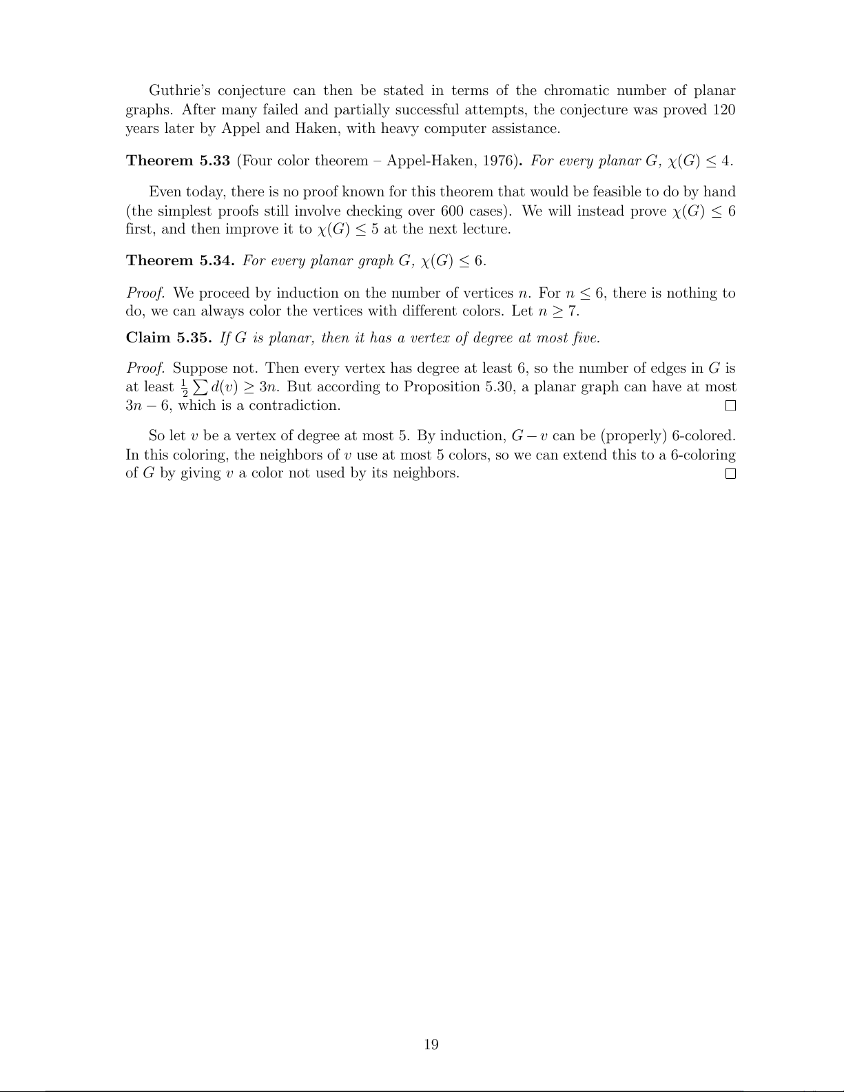
Guthrie’s conjecture can then be stated in terms of the chromatic number of planar
graphs. After many failed and partially successful attempts, the conjecture was proved 120
years later by Appel and Haken, with heavy computer assistance.
Theorem 5.33 (Four color theorem – Appel-Haken, 1976). For every planar G, χ(G) ≤ 4.
Even today, there is no proof known for this theorem that would be feasible to do by hand
(the simplest proofs still involve checking over 600 cases). We will instead prove χ(G) ≤ 6
first, and then improve it to χ(G) ≤ 5 at the next lecture.
Theorem 5.34. For every planar graph G, χ(G) ≤ 6.
Proof. We proceed by induction on the number of vertices n. For n ≤ 6, there is nothing to
do, we can always color the vertices with different colors. Let n ≥ 7.
Claim 5.35. If G is planar, then it has a vertex of degree at most five.
Proof. Suppose not. Then every vertex has degree at least 6, so the number of edges in G is
at least 1 P d(v) ≥ 3n. But according to Proposition 5.30, a planar graph can have at most 2
3n − 6, which is a contradiction.
So let v be a vertex of degree at most 5. By induction, G − v can be (properly) 6-colored.
In this coloring, the neighbors of v use at most 5 colors, so we can extend this to a 6-coloring
of G by giving v a color not used by its neighbors. 19 Lecture 6 Coloring. 1 Coloring planar graphs
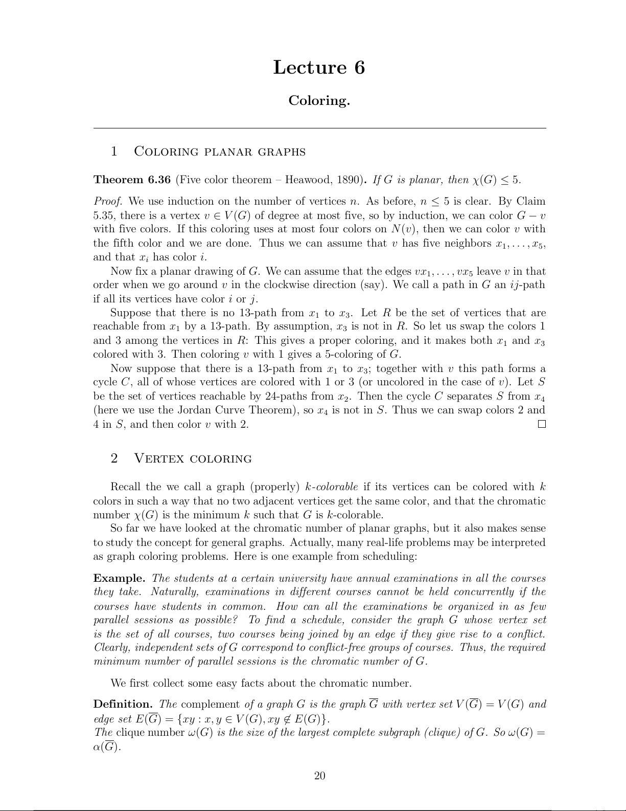
Theorem 6.36 (Five color theorem – Heawood, 1890). If G is planar, then χ(G) ≤ 5.
Proof. We use induction on the number of vertices n. As before, n ≤ 5 is clear. By Claim
5.35, there is a vertex v ∈ V (G) of degree at most five, so by induction, we can color G − v
with five colors. If this coloring uses at most four colors on N (v), then we can color v with
the fifth color and we are done. Thus we can assume that v has five neighbors x1, . . . , x5, and that xi has color i.
Now fix a planar drawing of G. We can assume that the edges vx1, . . . , vx5 leave v in that
order when we go around v in the clockwise direction (say). We call a path in G an ij-path
if all its vertices have color i or j.
Suppose that there is no 13-path from x1 to x3. Let R be the set of vertices that are
reachable from x1 by a 13-path. By assumption, x3 is not in R. So let us swap the colors 1
and 3 among the vertices in R: This gives a proper coloring, and it makes both x1 and x3
colored with 3. Then coloring v with 1 gives a 5-coloring of G.
Now suppose that there is a 13-path from x1 to x3; together with v this path forms a
cycle C, all of whose vertices are colored with 1 or 3 (or uncolored in the case of v). Let S
be the set of vertices reachable by 24-paths from x2. Then the cycle C separates S from x4
(here we use the Jordan Curve Theorem), so x4 is not in S. Thus we can swap colors 2 and
4 in S, and then color v with 2. 2 Vertex coloring
Recall the we call a graph (properly) k-colorable if its vertices can be colored with k
colors in such a way that no two adjacent vertices get the same color, and that the chromatic
number χ(G) is the minimum k such that G is k-colorable.
So far we have looked at the chromatic number of planar graphs, but it also makes sense
to study the concept for general graphs. Actually, many real-life problems may be interpreted
as graph coloring problems. Here is one example from scheduling:
Example. The students at a certain university have annual examinations in all the courses
they take. Naturally, examinations in different courses cannot be held concurrently if the
courses have students in common. How can all the examinations be organized in as few
parallel sessions as possible? To find a schedule, consider the graph G whose vertex set
is the set of all courses, two courses being joined by an edge if they give rise to a conflict.
Clearly, independent sets of G correspond to conflict-free groups of courses. Thus, the required
minimum number of parallel sessions is the chromatic number of G.
We first collect some easy facts about the chromatic number.
Definition. The complement of a graph G is the graph G with vertex set V (G) = V (G) and
edge set E(G) = {xy : x, y ∈ V (G), xy 6∈ E(G)}.
The clique number ω(G) is the size of the largest complete subgraph (clique) of G. So ω(G) = α(G). 20
Tài liệu liên quan:
-
Đề thi hết môn học kì Toán rời rạc năm học 2025-2026 - trường đại học Khoa học tự nhiên – Đại học quốc gia hà nội.
53 27 -
Đồ thị và đặc điểm cơ bản | Toán Rời Rạc | Trường Đại học Khoa học Tự nhiên, Đại học Quốc gia Hà Nội
146 73 -
Bài Tập Toán Rời Rạc: Chương 4 - Các Phương Pháp | Toán Rời Rạc | Trường Đại học Khoa học Tự nhiên, Đại học Quốc gia Hà Nội
135 68 -
Ôn tập Câu hỏi toán học nâng cao - Môn Toán | Toán Rời Rạc | Trường Đại học Khoa học Tự nhiên, Đại học Quốc gia Hà Nội
78 39 -
Phân Tích Các Bài Tập Xác Suất và Thống Kê | Toán Rời Rạc | Trường Đại học Khoa học Tự nhiên, Đại học Quốc gia Hà Nội
107 54