Lecture notes 15 - Math for business | Trường Đại học Quốc tế, Đại học Quốc gia Thành phố HCM

12/16/2021 Elliptic PDE - Introduction 12/16/2021 Son Dao, PhD (C) 1 1 Defining Elliptic PDE’s
 The general form for a second order linear PDE with two independent
variables ( ) and one dependent variable ( ) u is x , y 2 2 2  u  u  A  B  u C  D  0 2 2 x   x y y 
Recall the criteria for an equation of this type to be considered elliptic 2 B  4 AC  0
 For example, examine the Laplace equation given by 2 2  T   T  0 , where A 1  , B  0 , C  1 2 2 x y then 2 B 4 AC  0  ) 1 ( 4 ( ) 1  4  0
thus allowing us to classify this equation as elliptic. Son Dao, PhD (C) 2 2 1 12/16/2021
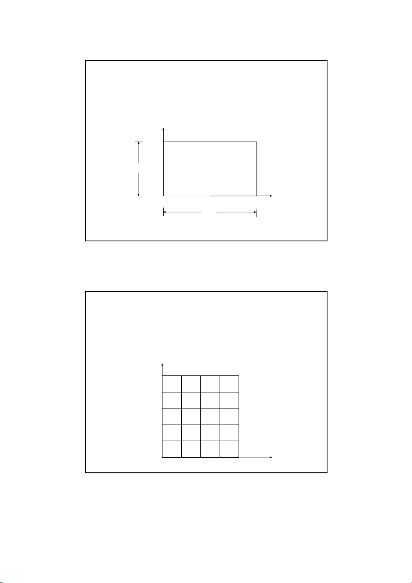
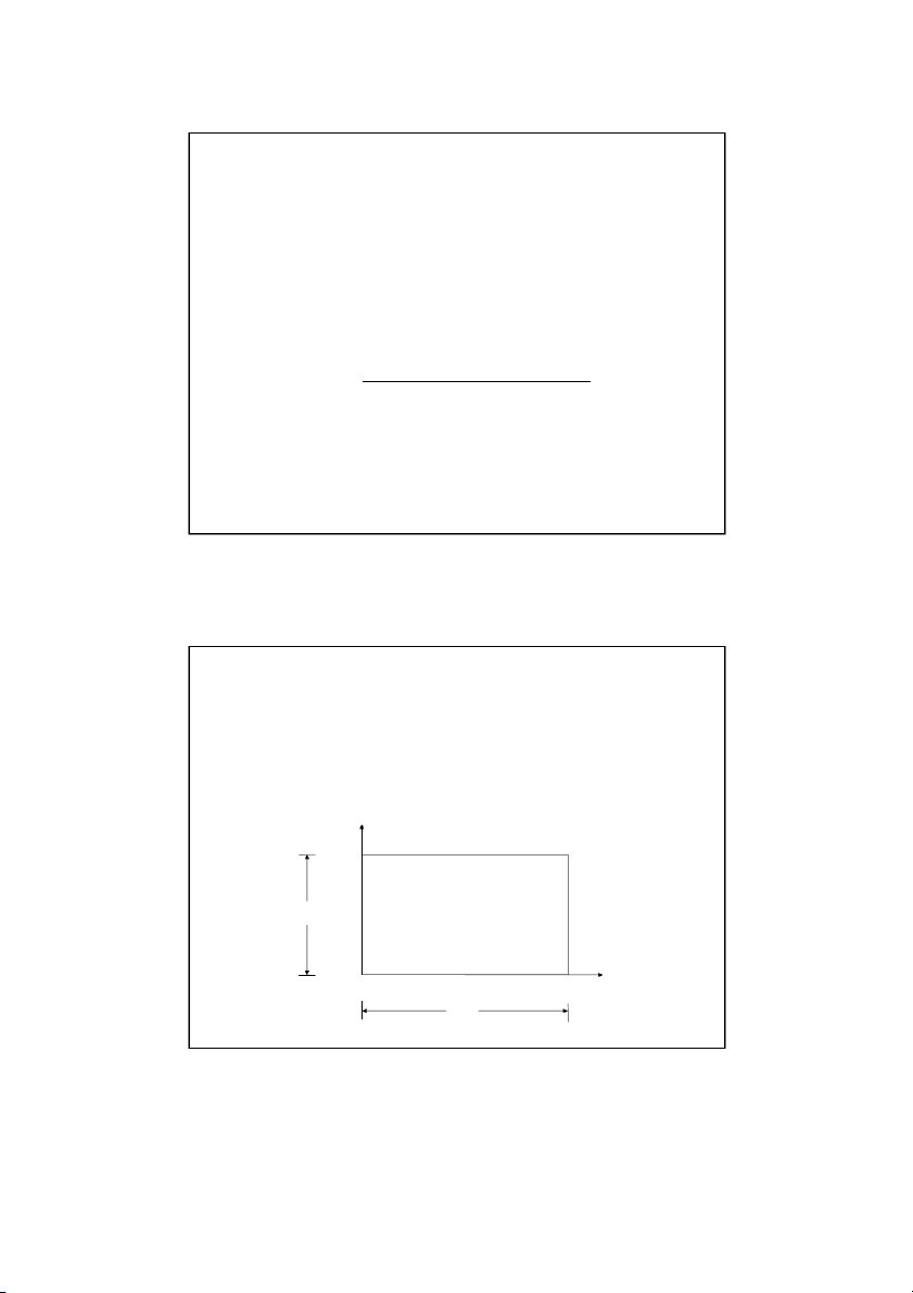
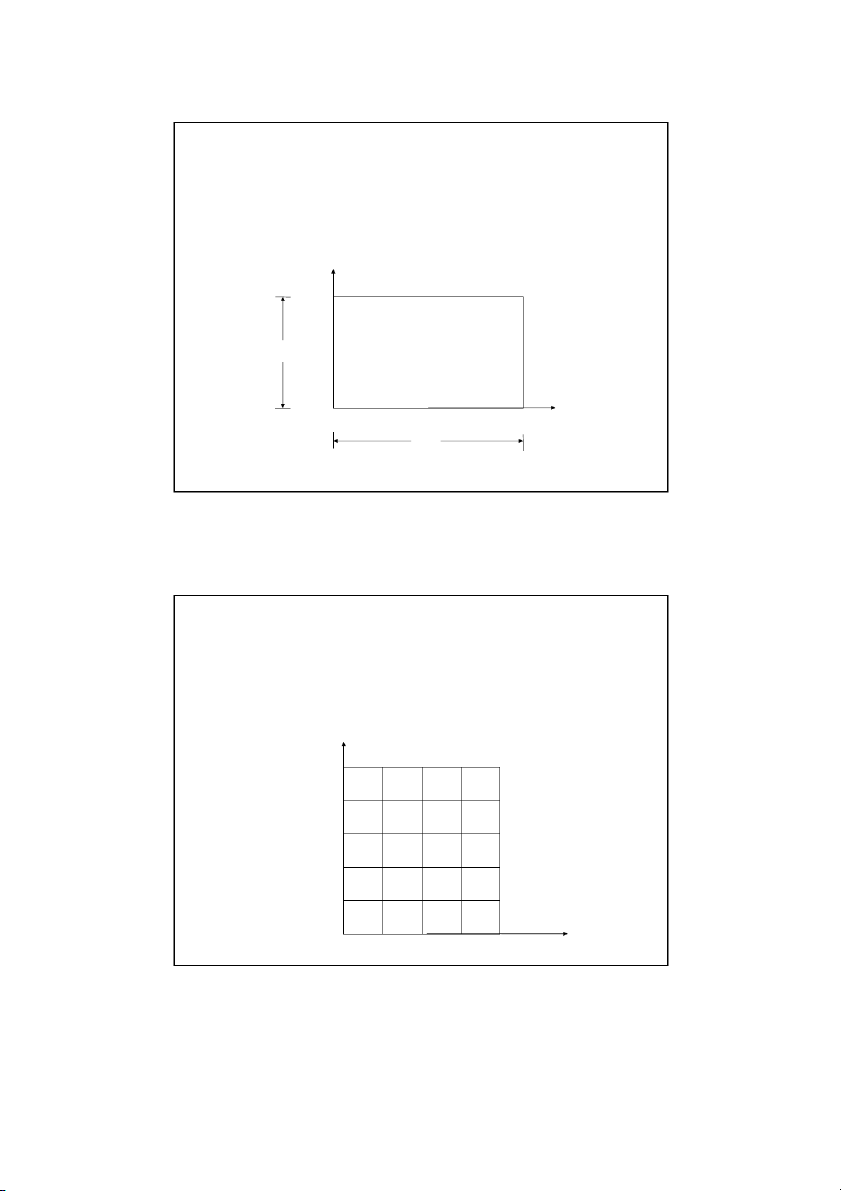
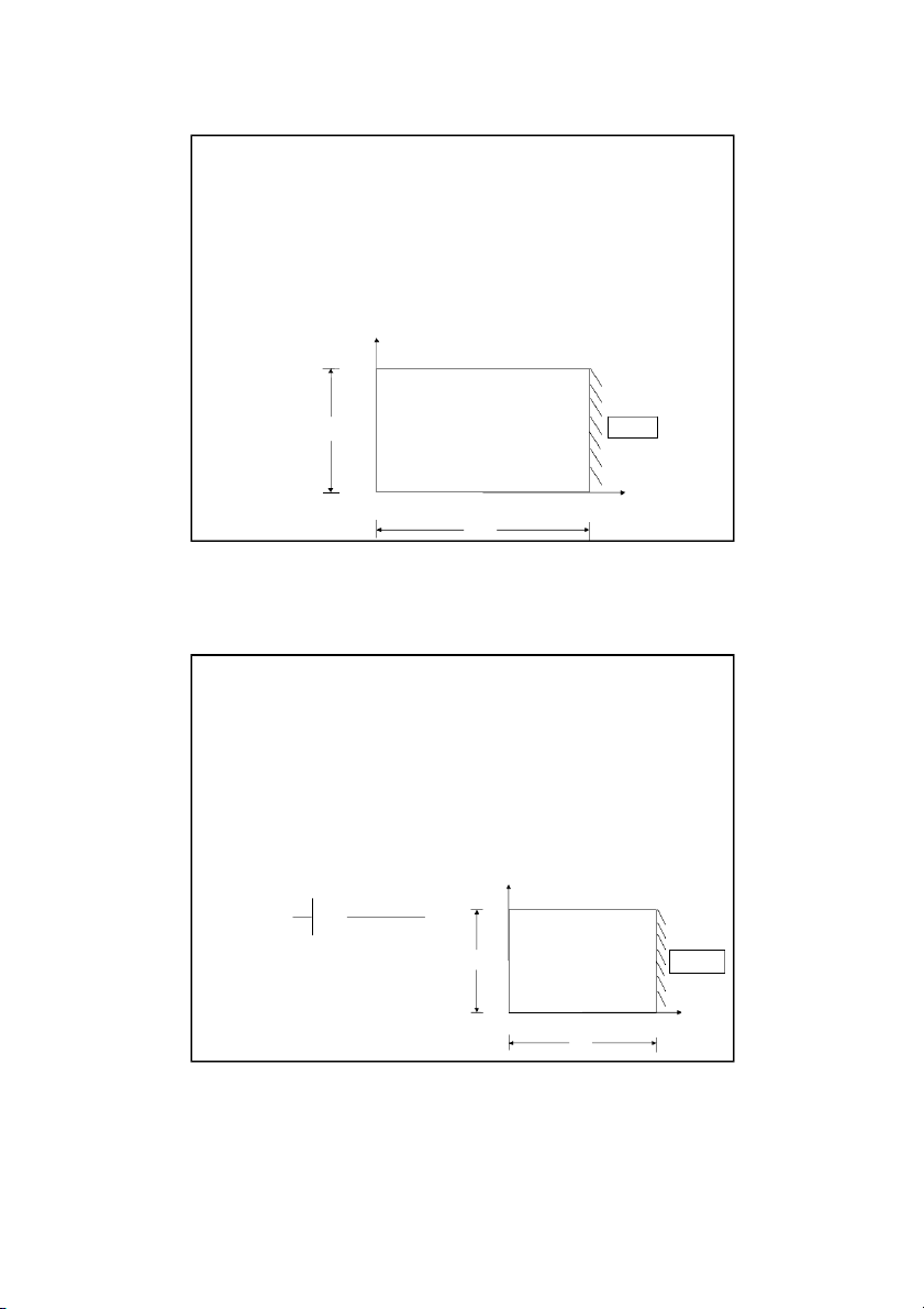
Physical Example of an Elliptic PDE y Tt W T T l r x Tb L
Schematic diagram of a plate with specified temperature boundary conditions 2 2  T  T
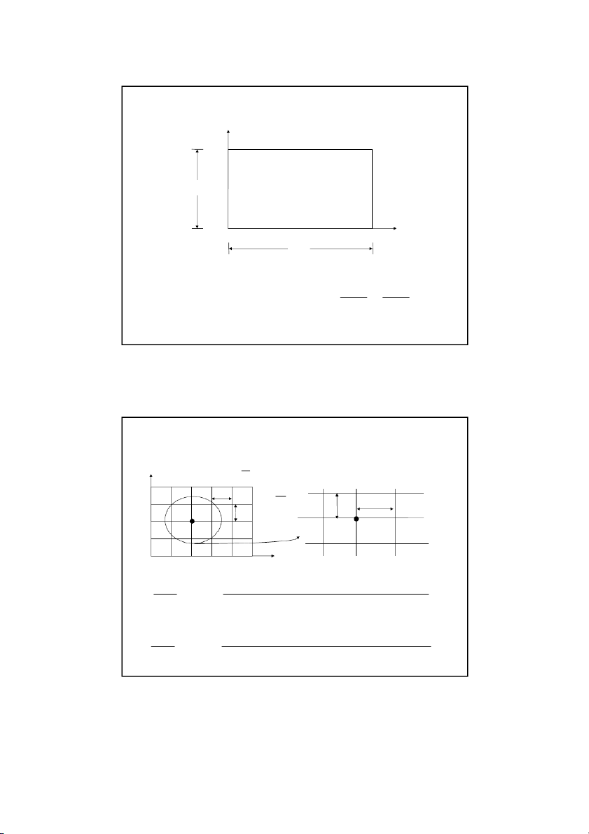
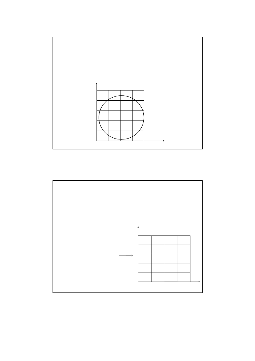
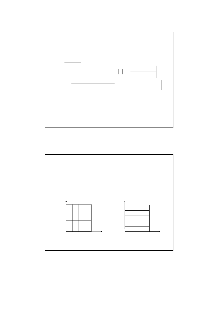
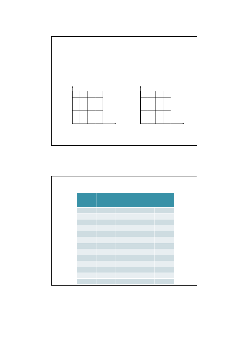
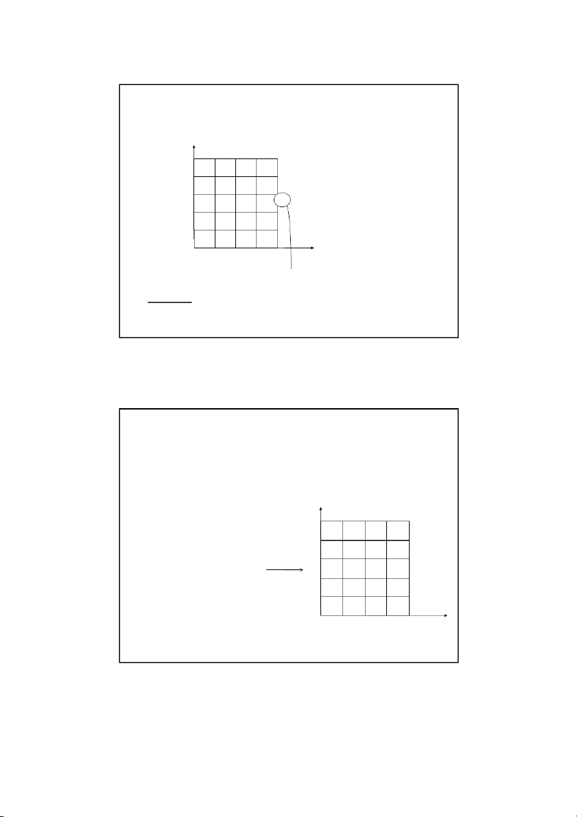
The Laplace equation governs the temperature:  0 2 2 x y Son Dao, PhD (C) 3 3 Discretizing the Elliptic PDE L y x  T m t , 0 ( n) W x  y  ( , i j  ) 1 n y  x  y  Tr (i  , 1 j) (i, j) (i , 1 j) l T (i, j) x ( , i j  ) 1 ) 0 , 0 ( Tb (m ) 0 , 2  T T (x  x
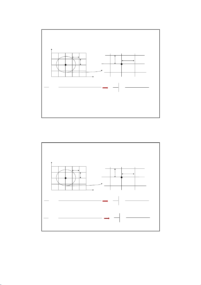
 , y)  2T (x, y) T (x  x  , y) (x, y )  2 x   2 x 2  T
T (x, y  y)  2T (x, y)  T (x, y  y  ) ( , x y)  2 y   y  2 Son Dao, PhD (C) 4 4 2 12/16/2021 Discretizing the Elliptic PDE y t T , 0 ( n) x  ( , i j  ) 1 y  x  y  r T T (i  , 1 j) (i, j) (i , 1 j) l (i, j) x ( , i j  ) 1 ) 0 , 0 ( T (m ) 0 , b 2 2  T T ( x   , x y)  2T( , x ) y  T( x   , x y)  T T   2T  T i , 1 j i, j i  , 1 j (x, y )   2 2 x   x  2 x x  ,  2 i j Son Dao, PhD (C) 5 5 Discretizing the Elliptic PDE y Tt , 0 ( n) x  ( , i j  ) 1 y  x  y  Tr (i  , 1 j) (i, j) (i , 1 j) l T (i, j) x ( , i j  ) 1 ) 0 , 0 ( Tb (m ) 0 , 2 2  T
T x  x y  T x y  T x  x y T ( , ) 2 ( , ) ( , )  T  2T  T i  , 1 j i, j i  , 1 j (x, y )   2 2 x   x  2 x  x  2 , i j 2 2 T  T
T (x , y  y ) 2T (x , y ) T (x , y  y )  T  2T  T i, j 1  i, j i, j 1 ( , x ) y    2 2  y  y  2 y y 2 i , j Son Dao, PhD (C) 6 6 3 12/16/2021 Discretizing the Elliptic PDE 2 2  T   T  0 2 2 x  y
Substituting these approximations into the Laplace equation yields: T  2T  T T  2T  i  T , 1 j i, j i  , 1 j , i j 1  , i j , i j 1     2 x y 0 2 if, x   y 
the Laplace equation can be rewritten as T  T T T  4T  0 i , 1 j i , 1 j i, j 1  i , j 1  i, j Son Dao, PhD (C) 7 7 Discretizing the Elliptic PDE T  T  T  T  4T  0 i  , 1 j i , 1 j i , j 1  i , j 1  i , j
Once the governing equation has been
discretized there are several numerical
methods that can be used to solve the problem. We will examine the: •Direct Method •Gauss-Seidel Method •Lieberman Method Son Dao, PhD (C) 8 8 4 12/16/2021 Example 1: Direct Method Consider a plate 2 . 4 m  3 . 0
m that is subjected to the boundary conditions
shown below. Find the temperature at the interior nodes using a square grid with a length of 0 6 . m by using the direct method. y 300 C  75 C 100 C  3.0 m x 50C 2 4 . m Son Dao, PhD (C) 9 9 Example 1: Direct Method
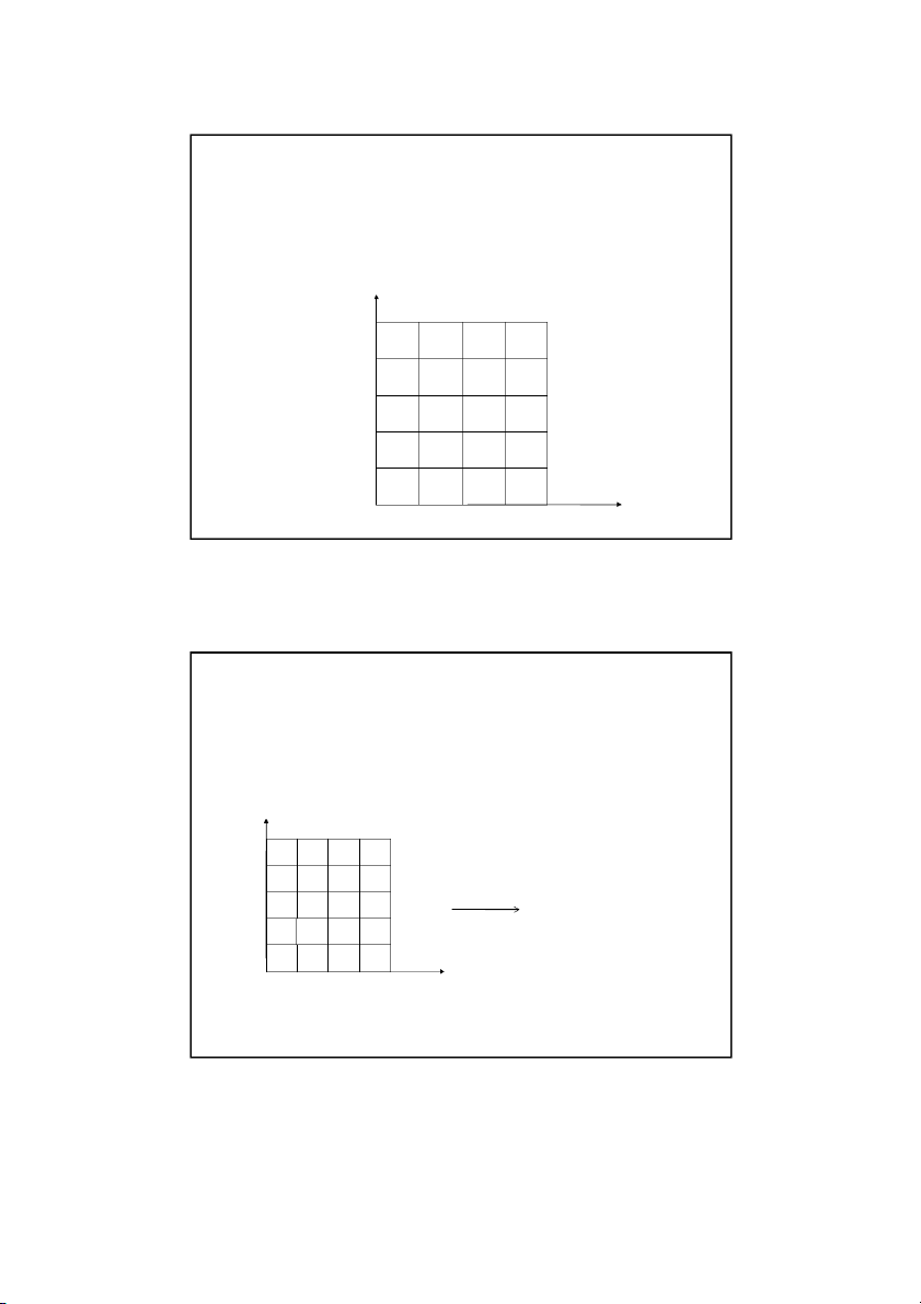
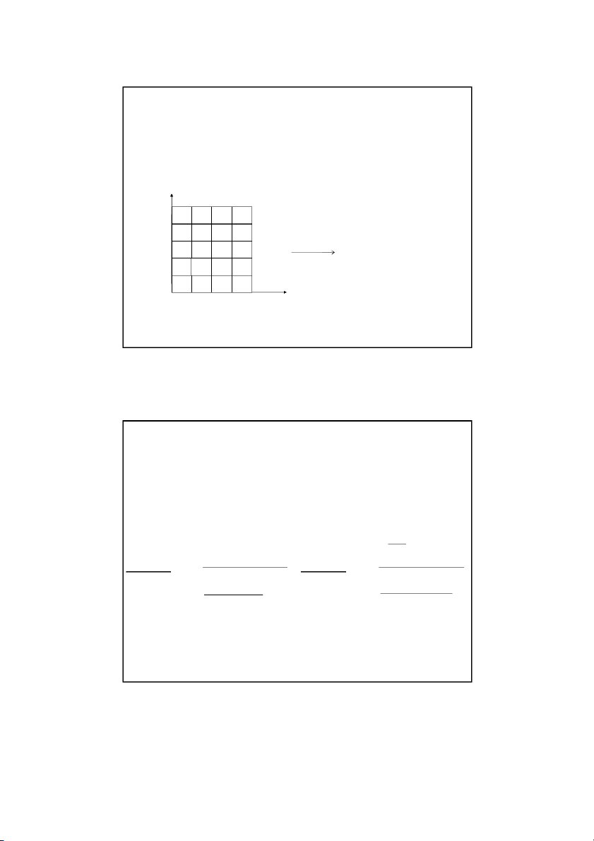
We can discretize the plate by taking, x   y   6 . 0 m Son Dao, PhD (C) 10 10 5 12/16/2021 Example 1: Direct Method
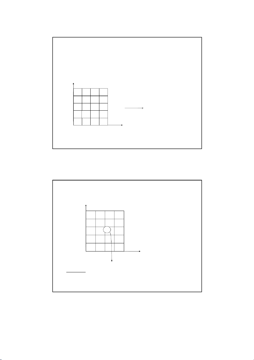
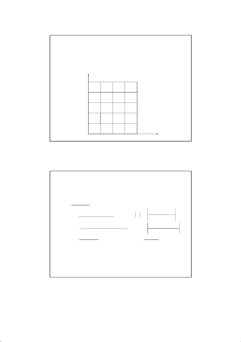
The nodal temperatures at the boundary nodes are given by: 30  y 0 C T T T T T , 1 5 2,5 , 3 5 4,5 0,5 T  7 , 5 j  , 1 , 3 , 2 4 T 0, j 0,4 T T T T , 1 4 2,4 3,4 4,4 T 10 , 0 j  , 1 2 , 3 , 4 T 100 C  4,j 0,3 75 C  T T T T , 1 3 2,3 , 3 3 4,3 T T  5 , 0 i  , 1 3 , 2 0,2 , i 0 T T T T , 1 2 2,2 3,2 4,2 T  30 , 0 i  , 1 3 , 2 T , i 5 0 1 , T T T T 1 , 1 2 1 , 3 1 , 4 1 , x T0,0 T T T T , 1 0 2,0 , 3 0 4,0 50 C  Son Dao, PhD (C) 11 11 Example 1: Direct Method y T T T T , 1 T 5 2,5 , 3 5 4,5 0,5 T0,4 , 1 T 4 T2,4 T T 3,4 4,4 0 T ,3 , 1 T 3 2 T,3 T ,33 T4,3 0 T ,2 , 1 T 2 T T T 2,2 3,2 4,2 0 T 1, T T T T 1 , 1 2 1 , 1 , 3 4 1 , x T0,0 T T T , 1 T 0 2,0 3,0 4,0
Here we develop the equation for the temperature at the node (2,3) i=2 and j=3 T  T  T  T T i j i j i j  i j  4  0  , 1 , 1 , 1 , 1 , i j T  T  T  T  4T  0 , 3 3 , 1 3 2, 4 2,2 , 2 3 T  T  4T T T  0 , 1 3 2,2 2,3 2,4 3,3 Son Dao, PhD (C) 12 12 6 12/16/2021 Example 1: Direct Method
We can develop similar equations for every interior node leaving us
with an equal number of equations and unknowns.
Question: How many equations would this generate? Son Dao, PhD (C) 13 13 Example 1: Direct Method
We can develop similar equations for every interior node leaving us
with an equal number of equations and unknowns.
Question: How many equations would this generate? Answer: 12 y  T  1 , 1 73 8 . 92  4   T    300 300 300 , 1 2  9 . 3 025  2 T  119 9 . 0  7  ,13    T  ,14  173 3 . 5  5 75 100  173 182 T    77 5 . 443 199  1, 2   
Solving yields:  T2,2  103 3 . 0  2 100   C 75  120 138 131 T     2,3  138 2 . 4  8 T 75 100 2,4  198 5 . 1  2   93 103 104 T    1, 3  82 9 . 83  3 T  104 3 . 8  9 75 100 74 78 83  3,2    T  ,33  13 . 1 27  1 x T  182 4 . 4   3,4    6 50 50 50 Son Dao, PhD (C) 14 14 7 12/16/2021 The Gauss-Seidel Method
 Recall the discretized equation T  T  T  T  4T  0 i  , 1 j i , 1 j , i j 1  i, j 1  i, j  This can be rewritten as T  T  T  T i  , 1 j i  , 1 j i, j 1  i , 1  T  j i , j 4
 For the Gauss-Seidel Method, this
equation is solved iteratively for all
interior nodes until a pre-specified tolerance is met. Son Dao, PhD (C) 15 15 Example 2: Gauss-Seidel Method Consider a plate 2 . 4 m  3 . 0
m that is subjected to the boundary conditions
shown below. Find the temperature at the interior nodes using a square grid with a length of 0 6 .
m using the Gauss-Siedel method. Assume the
initial temperature at all interior nodes to be 0  C . y 300 C  75 C 100 C  3.0 m x 50 C . 2 4 m Son Dao, PhD (C) 16 16 8 12/16/2021 Example 2: Gauss-Seidel Method
We can discretize the plate by taking x   y  6 . 0 m Son Dao, PhD (C) 17 17 Example 2: Gauss-Seidel Method
The nodal temperatures at the boundary nodes are given by: 300  y C T T T T T , 1 5 2,5 , 3 5 4,5 0,5 T  7 , 5 j  , 1 , 3 , 2 4 T 0, j , 0 4 T T , 1 4 2,4 T T , 3 4 4,4 T 100 C  10 , 0 j  , 1 2 , 3 , 4 T0,3 4,j 75 C  T T T , 1 3 2,3 , 3 T 3 4,3 T T  5 , 0 i  , 1 3 , 2 , 0 2 , i 0 T T T T , 1 2 2,2 , 3 2 4,2 T  30 , 0 i  , 1 3 , 2 T0 1, T T T T , i 5 1 , 1 2 1 , 3 1 , 4 1 , x T0,0 T T T T , 1 0 2,0 , 3 0 4,0 50 C  Son Dao, PhD (C) 18 18 9 12/16/2021 Example 2: Gauss-Seidel Method
•Now we can begin to solve for the temperature at each interior node using T T T T i j  i j  i j   , 1  , 1 , 1  i, 1 T  j , i j 4
•Assume all internal nodes to have an initial temperature of zero. Iteration #1 T T T T i=1 and j=1 1 , 2 0 1 , , 1 2 , 1 0 T  1 , 1 4 0  75  0  50  4  31 2 . 50  0 C T  T  T  T i=1 and j=2 2,2 0,2 1,3 1 , 1 T  1,2 4 0  75 0 3 . 1 2500  4  26 5 . 625 C  Son Dao, PhD (C) 19 19 Example 2: Gauss-Seidel Method
After the first iteration, the temperatures are as follows. These will now be
used as the nodal temperatures for the second iteration. y 300 C  100 102 135 25 9 3 . 37 75  C 100 C  27 12 39 31 20 43 x 50 C  Son Dao, PhD (C) 20 20 10 12/16/2021 Example 2: Gauss-Seidel Method Iteration #2 i=1 and j=1 present T  previous T T T T T 1 , 1 1 , 1 2 1 , 0 1 , , 1 2 , 1 0    T  100 a 1 , 1 1 , 1 present 4 T 1, 1 20 3 . 125 75 26 5 . 625  50  42 9 . 688 31 2 . 500  1  00 4 42 9 . 688  42 9 . 68  8 C  27 2 . % 7 Son Dao, PhD (C) 21 21 Example 2: Gauss-Seidel Method
The figures below show the temperature distribution and absolute
relative error distribution in the plate after two iterations: Absolute Relative Approximate Temperature Distribution Error Distribution y y 300 300 300 75 133 156 161 100 25% 3 % 4 1 % 6 75 56 56 87 100 5 % 4 83% 5 % 8 75 39 29 56 100 3 % 1 62% 3 % 2 75 43 37 56 100 2 % 7 45% 24% x x 50 50 50 Son Dao, PhD (C) 22 22 11 12/16/2021 Example 2: Gauss-Seidel Method
Temperature Distribution in the Plate (°C) Node Number of Iterations 1 2 10 Exact T 1, 1 31.2500 42.9688 73.0239 T ,12 26.5625 38.7695 91.9585 T ,13 25.3906 55.7861 119.0976 T ,14 100.0977 133.2825 172.9755 T 1, 2 20.3125 36.8164 76.6127 T2,2 11.7188 30.8594 102.1577 T2,3 9.2773 56.4880 137.3802 T2,4 102.3438 156.1493 198.1055 T 1, 3 42.5781 56.3477 82.4837 T3,2 38.5742 56.0425 103.7757 T3,3 36.9629 86.8393 130.8056 T3,4 134.8267 160.7471 182.2278 Son Dao, PhD (C) 23 23 The Lieberman Method
 Recall the equation used in the Gauss- Siedel Method, T  T  T  T i , 1 j i , 1 j , i j 1  i, 1  T  j i, j 4
 Because the Guass-Siedel Method is
guaranteed to converge, we can accelerate
the process by using over- relaxation. In this case, relaxed new old T  T  1 (   T ) i, j i, j i ,j Son Dao, PhD (C) 24 24 12 12/16/2021 Example 3: Lieberman Method Consider a plate 2 . 4 m  3 . 0
m that is subjected to the boundary conditions
shown below. Find the temperature at the interior nodes using a square grid with a length of 0 6 .
m . Use a weighting factor of 1.4 in the Lieberman
method. Assume the initial temperature at all interior nodes to be 0 C  . y 300 C  75 C 100 C  3.0 m x 50 C . 2 4 m Son Dao, PhD (C) 25 25 Example 3: Lieberman Method
We can discretize the plate by taking x   y   6 . 0 m Son Dao, PhD (C) 26 26 13 12/16/2021 Example 3: Lieberman Method
We can also develop equations for the boundary conditions to define the
temperature of the exterior nodes. 300  y C T T T T T , 1 5 2,5 , 3 5 4,5 0,5 T  7 , 5 j  , 1 , 3 , 2 4 T 0, j , 0 4 T T T T , 1 4 2,4 , 3 4 4,4 T 10 , 0 j  , 1 2 , 3 , 4 T 100 C  4,j 0,3 75 C  T T T T , 1 3 2,3 , 3 3 4,3 T T  5 , 0 i  , 1 3 , 2 , 0 2 , i 0 T T T T , 1 2 2,2 , 3 2 4,2 T  30 , 0 i  , 1 3 , 2 T , i 5 0 1 , T T T T 1 , 1 2 1 , 3 1 , 4 1 , x T0,0 T T T T , 1 0 2,0 , 3 0 4,0 50 C Son Dao, PhD (C) 27 27 Example 3: Lieberman Method
•Now we can begin to solve for the temperature at each interior node using
the rewritten Laplace equation from the Gauss-Siedel method.
•Once we have the temperature value for each node we will apply the over
relaxation equation of the Lieberman method
•Assume all internal nodes to have an initial temperature of zero. Iteration #1 Iteration #2 T  T  T  T T T  T T 1 , 2 1 , 0 , 1 2 , 1 0 2, 2 0,2 , 1 3 1 , 1 i=1 and j=1 T  T  1 , 1 i=1 and j=2 , 1 2 4 4 0  75  0  50 0  75 0  43 7 . 5   4 4  31 2 . 500 C   29 6 . 875 C  relaxed new   (1 ) old T T T relaxed new    (1 ) old T T T 1,1 1,1 1,1 1,1 1,1 1,1  4 . 1 3 ( 1 2 . 50 ) 0  1 (  ) 4 . 1 0  4 . 1 (29 6 . 87 ) 5  1 (  ) 4 . 1 0  4 . 3 7500 C   4 . 1 5625 C  Son Dao, PhD (C) 28 28 14 12/16/2021 Example 3: Lieberman Method
After the first iteration the temperatures are as follows. These will be used
as the initial nodal temperatures during the second iteration. y 300 C  146 164 221 41 23 66 75  C 100 C  42 26 67 44 33 64 x 50 C  Son Dao, PhD (C) 29 29 Example 3: Lieberman Method Iteration #2 i=1 and j=1 present T  previous T T T T T 1 , 1 1 , 1 2 1 , 0 1 , , 1 2 , 1 0    T  100 a 1 , 1 present 1 , 1 T 4 1 , 1 3 . 2 8125 75 41 5 . 625  52 2 . 813 43 7 . 500  50  100 4 52 2 . 813  49 8 . 438 C   16 3 . % 2 relaxed new  (1   ) old T T T 1,1 1,1 1,1  ( 4 . 1 4 . 9 843 ) 8  1 (  ) 4 . 1 43 7 . 5  5 . 2 2813 C  Son Dao, PhD (C) 30 30 15 12/16/2021 Example 3: Lieberman Method
The figures below show the temperature distribution and absolute
relative error distribution in the plate after two iterations: Absolute Relative Temperature Distribution Approximate Error Distribution y y 300 300 300 75 161 9. % 6 216 181 100 2 % 4 2 % 2 75 87 122 155 100 5 % 3 8 % 1 5 % 7 75 51 58 76 100 1 % 9 5 % 5 1 % 3 75 52 54 69 100 1 % 6 3 % 9 7 5 . % x x 50 50 50 Son Dao, PhD (C) 31 31 Example 3: Lieberman Method
Temperature Distribution in the Plate (°C) Node Number of Iterations 1 2 9 Exact T 1, 1 43.7500 52.2813 73.7832 T ,12 41.5625 51.3133 92.9758 T ,13 40.7969 87.0125 119.9378 T ,14 145.5289 160.9353 173.3937 T 1, 2 32.8125 54.1789 77.5449 2 T ,2 26.0313 57.9731 103.3285 T2,3 23.3898 122.0937 138.3236 T2,4 164.1216 215.6582 198.5498 T 1, 3 63.9844 69.1458 82.9805 T3,2 66.5055 76.1516 104.3815 T3,3 66.4634 155.0472 131.2525 T Son Dao, PhD (C) 32 3,4 220.7047 181.4650 182.4230 32 16 12/16/2021
Alternative Boundary Conditions
 In Examples 1-3, the boundary conditions on the plate had a
specified temperature on each edge. What if the conditions are
different ? For example, what if one of the edges of the plate is insulated.
 In this case, the boundary condition would be the derivative of
the temperature. Because if the right edge of the plate is
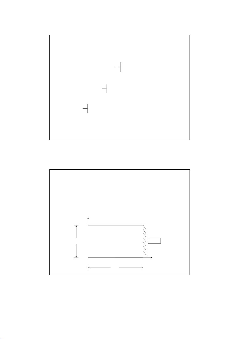
insulated, then the temperatures on the right edge nodes also become unknowns. y 300C 75 C  0 . 3 m Insulated x 50 C  4 . 2 m Son Dao, PhD (C) 33 33
Alternative Boundary Conditions
 The finite difference equation in this case for the right edge for the nodes ( m , j ) for j  3 , 2 , . . n 1 T  T  T  T  4T  0  m , 1 j m , 1 j m, j 1  , m j 1  m, j  However the node ( m  , 1 j
) is not inside the plate. The
derivative boundary condition needs to be used to account for
these additional unknown nodal temperatures on the right edge.
This is done by approximating the derivative at the edge node as (m, j) y 300C  T  T   m , 1 T j m  , 1 j   x ( 2 x  ) , m j 7  5 C m 0 . 3 Insulated x 5  0 C . 2 m 4 Son Dao, PhD (C) 34 34 17 12/16/2021
Alternative Boundary Conditions
 Rearranging this approximation gives us, T  T   2( )  , 1 T  ,1 x m j m j  x m,j
 We can then substitute this into the original equation gives us, T 2T  ( 2  ) x  T  T  4T  0  m , 1 j m, j 1  m, j 1  m,  j x , m j
 Recall that is the edge is insulated then, T  0 x ,m j
 Substituting this again yields, 2T  T  T  4T  0 m 1  , j m , j 1  m , j 1  m, j Son Dao, PhD (C) 35 35 Example 3: Alternative Boundary Conditions A plate 4 . 2 m  0 . 3
m is subjected to the temperatures and insulated boundary
conditions as shown in Fig. 12. Use a square grid length of . 0 6 m . Assume the
initial temperatures at all of the interior nodes to be 0 C  . Find the temperatures
at the interior nodes using the direct method. y 300 C  75 C  0 . 3 m Insulated x 50 C  4 . 2 m Son Dao, PhD (C) 36 36 18 12/16/2021 Example 3: Alternative Boundary Conditions
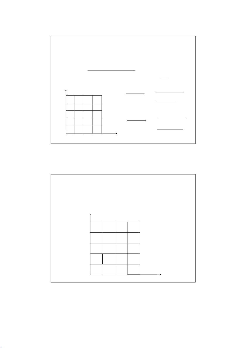
We can discretize the plate taking, x y  . 0 6m Son Dao, PhD (C) 37 37 Example 3: Alternative Boundary Conditions
We can also develop equations for the boundary conditions to define the
temperature of the exterior nodes. 30  y 0 C T T T T T , 1 5 2,5 , 3 5 4,5 0,5 T  7 ; 5 j  , 3 , 2 , 1 4 0, j T ,04 T T T  5 ; 0 i  , 1 , 3 , 2 4 , 1 4 2,4 T T , 3 4 4,4 i ,0 T0,3 75 C  T T T Insulated T  i  , 1 3 2,3 , 3 T 3 30 ; 0 , 1 , 3 , 2 4 4,3 i ,5 T ,02 T T T T , 1 2 2,2 , 3 2 4,2 T  ; 0 j  , 3 , 2 , 1 4 T0 1, T T T T 1 , 1 2 1 , 3 1 , 4 1 , x x 4, j T0,0 T T T T , 1 0 2,0 , 3 0 4,0 50 C  Son Dao, PhD (C) 38 38 19 12/16/2021 Example 3: Alternative Boundary Conditions y T T T , 1 5 2 T ,5 , 3 5 4 T ,5 , 0 5 T0,4 T T 1,4 2,4 T T , 3 4 4,4 T0,3 T T T , 1 3 2,3 3,3 T4,3 T0,2 T T T T 1,2 2,2 3,2 4,2 T0,1 T T T T , 1 1 2,1 3,1 4,1 x T0,0 , 1 T 0 T T T 2,0 , 3 0 4,0
Here we develop the equation for the temperature at the node (4,3),
to show the effects of the alternative boundary condition. i=4 and j=3 2 T  T  T 4  T 0  , 3 3 , 4 2 4,4 4,3 2T T  4T  T  0 3,3 4,2 4,3 4,4 Son Dao, PhD (C) 39 39 Example 3: Alternative Boundary Conditions
The addition of the equations for the boundary conditions gives us a
system of 16 equations with 16 unknowns. T1, 1  76 8 . 25  4     T  ,12  99 4 . 444 y T  , 1 3 12 . 8 617     300 300 300 T  ,14  180 4 . 10 T    2 1 , 82 8 . 57    1   T 75  2,2 11 . 7 335 180 218 232 233 T      2,3 159 6 . 14 75 Solving yields: T   129 160 174 179 2,4 21 . 8 021      C  T  3 1, 87 2 . 678 75 T   99 117 127 131 , 3 2 127 4 . 26     T 75  3,3 174 4 . 83 77 T  83 87 89 3,4      23 . 2 060   x T  4 1,  88 7 . 882 50 50 50 T      4,2 13 . 0 617 T   4,3 178 8 . 30     T  4,4 23 . 2 738 Son Dao, PhD (C) 40 40 20