Lecture notes 16 - Math for business | Trường Đại học Quốc tế, Đại học Quốc gia Thành phố HCM

12/16/2021 Parabolic PDE 12/16/2021 1 Son Dao, PhD © 1 1 Defining Parabolic PDE’s
 The general form for a second order linear PDE with two independent
variables and one dependent variable is 2 2 2  u  u  A  B  u C  D  0 2 2 x   x y y 
Recall the criteria for an equation of this type to be considered parabolic 2 B  4 AC  0
 For example, examine the heat-conduction equation given by  2 T T    , where A  , B  , 0 C  , 0 D  1  x  2 t  Then 2 B  4AC  0  4( )(0)  0
thus allowing us to classify this equation as parabolic. Son Dao, PhD © 2 2 1 12/16/2021
Physical Example of an Elliptic PDE
The internal temperature of a metal rod exposed to two different
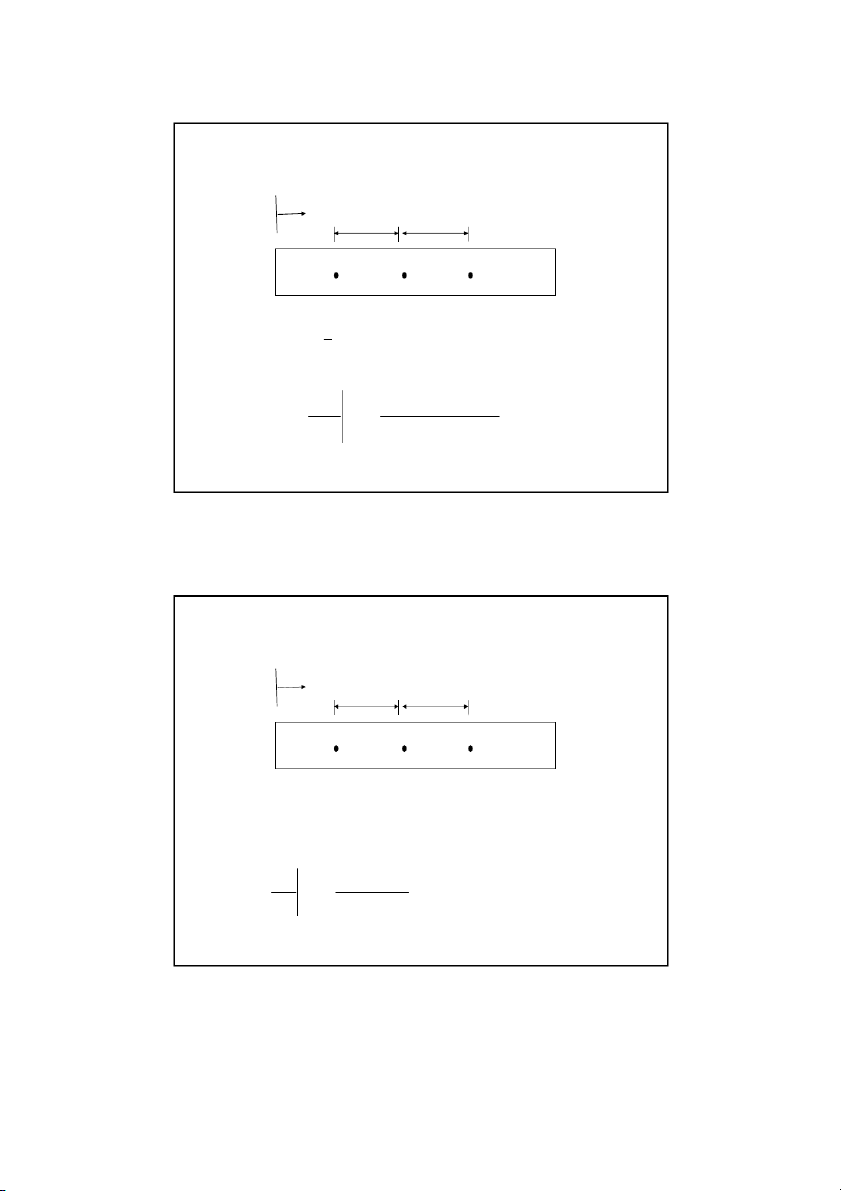
temperatures at each end can be found using the heat conduction equation.  T 2 T    x  2 t  Son Dao, PhD © 3 3 Discretizing the Parabolic PDE x x x i 1 i i  1
Schematic diagram showing interior nodes L For a rod of length L divided into n  1 nodes x  n
The time is similarly broken into time steps of t Hence
T j corresponds to the temperature at node i ,that is, i x  i x
  and time t   j t   Son Dao, PhD © 4 4 2 12/16/2021 The Explicit Method x x x i 1 i i  1 L If we define x  
we can then write the finite central divided difference n
approximation of the left hand side at a general interior node ( i ) as 2  T T j  2T j  T j i 1 i i1  2 x  x2 i , j
where ( j ) is the node number along the time. Son Dao, PhD © 5 5 The Explicit Method x x x i 1 i i  1
The time derivative on the right hand side is approximated by the
forward divided difference method as, T  T j1  T j i i  t t i, j Son Dao, PhD © 6 6 3 12/16/2021 The Explicit Method
Substituting these approximations into the governing equation yields T j 1   T j 2 T j T j  T j i 1 i i1 i i    x2 t
Solving for the temp at the time node j  1 gives  1  t j j T  T   T  T   2 T i i  j j j 2 i 1 i i 1   (x) choosing, t    2 ( x) we can write the equation as, j 1  j T T   T  T 2 T i i  j j j i 1  i i 1   . Son Dao, PhD © 7 7 The Explicit Method j 1  j T  T   T  2T  T i i  j j j i 1 i i1 
•This equation can be solved explicitly because it can be written for each
internal location node of the rod for time node j 1  in terms of the temperature at time node j.
•In other words, if we know the temperature at node j  0 , and the
boundary temperatures, we can find the temperature at the next time step.
•We continue the process by first finding the temperature at all nodes j  1 ,
and using these to find the temperature at the next time node, j  2 . This
process continues until we reach the time at which we are interested in finding the temperature. Son Dao, PhD © 8 8 4 12/16/2021 Example 1: Explicit Method
Consider a steel rod that is subjected to a temperature of 1 0 0 C  on the left end and 2 5 C
 on the right end. If the rod is of length . 0 0 5 m ,use the explicit
method to find the temperature distribution in the rod from t  0 and t  9 seconds. Use  x  0 . 0 1 m ,  t  3 s. kg J Given:  54 W k ,   7 8 0 0 , C  490 m  K 3 m kg  K
The initial temperature of the rod is 2 0 C  . i  0 1 2 3 4 5 T 10  0 C T 25 C  0 0 . m 1 Son Dao, PhD © 9 9 Example 1: Explicit Method Recall, Number of time steps, k t  t   final initial  C  t 9 0 therefore,  3 54    7800  490 3. 1 4 . 129 10 5   m2 / s. Boundary Conditions j T  100 C Then, 0 j  for all j  , 1 , 0 3 , 2 t     T  C  5 25    2 x 3 5  1 4 . 129 10  All internal nodes are at 2 0 C  0.012 for t  0 s e c . This can be  0 4 . 239. represented as, 0 T  20C, for a l li  1,2,3,4 i Son Dao, PhD © 10 10 5 12/16/2021 Example 1: Explicit Method Nodal temperatures when t  0 se c , j  0: T 0  100 C  0 0 T  20 C 1  0 T  20 C 2 I  nterior n odes 0 T  20 C 3  0 T  20  C 4  T 0  25 C  5
We can now calculate the temperature at each node explicitly using
the equation formulated earlier, j 1  j T  T   T  T 2 T i i  j j j i 1  i i 1   Son Dao, PhD © 11 11 Example 1: Explicit Method Nodal temperatures when t  3 s e c (Example Calculations) 1 i  0
T  100C  Boundary Condition 0 setting j  0 i  1 T 1  i  2 T1  T0   2 2 T0  T 2 0  T 0 3 2 1  1  T 0 1  T 02  T 2 0 1 T 0 0   20 0 4 . 239 20  ( 2 2 ) 0  100   20  0 4 . 23920  ( 2 20)  20  20  0.4239 80   20  0 4 . 23  9  0  20 33.912  20  0  53.  912 C  20 C  Nodal temperatures when t  3 s e c , j  1 : 1 T  C  0 100 Boundary Condition 1 T  5 . 3 912C  1  1 T  20C 2   I nterior n odes 1 T  20C 3  1  T  2 . 2 120C 4  1
T  25C  Boundary Condition 5 Son Dao, PhD © 12 12 6 12/16/2021 Example 1: Explicit Method Nodal temperatures when t  6 s e c (Example Calculations) 2 i  0
T  100C  Boundary Condition 0 setting j  1 , i  1 T 2  T 1   T 2  T 1   2 2 T1  T 2 1  T 1 3 2 1  1 1 T 1 T 2  1 T 1 2 1 0  i  2 53.912  . 0 423  9 20  ( 2 53 9 . 12) 10  0  20  . 0 423920 2(20)  5 . 3 912   5 . 3 912  . 0 423  9 1 . 2 176  20 . 0 42393 . 3 912  53.912  . 5 1614  20  1 . 4 375  5 . 9 07  3 C  3 . 4 375 C Nodal temperatures when t  6 s e c , j  2 : 2 T  C  0 100 Boundary Condition 2 T  5 . 9 073C 1  2 T  3 . 4 375C 2   I nterior n odes 2 T  2 . 0 889C 3  2 T  2 . 2 442  C 4  2
T  25C  Boundary Condition 5 Son Dao, PhD © 13 13 Example 1: Explicit Method Nodal temperatures when t  9 s e c (Example Calculations) 3 i  0
T  100C  Boundary Condition 0 setting j  2 , i  1 i  2 T 3  T 2   T 3  2  T 2 2  T 23 2T 22T21  1 1 T2  2T 2 T2 2 1 0   59 0 . 73  . 0 423  9 34 3 . 75 2(5 . 9 07 ) 3 100  34 3 . 75  0 4 . 23  9 20.899  2 3 ( 4 3 . 7 ) 5  59.07  3  5 . 9 073  . 0 423  9 1 . 6 229  34 3 . 75  0.4239 1 . 1 222  59.073  . 6 8795  34 3 . 75  4 7 . 570  6 . 5 953 C   3 . 9 132 C  Nodal temperatures when t  9 s e c , j  3 : 3 T  C  0 100 BoundaryCondition 3 T  6 . 5 953C 1  3 T  3 . 9 132C 2   I nterior n odes 3 T  2 . 7 266C 3  3  T  2 . 2 872C 4  3
T  25C  Boundary Condition 5 Son Dao, PhD © 14 14 7 12/16/2021 Example 1: Explicit Method
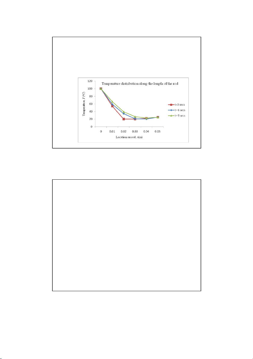
To better visualize the temperature variation at different
locations at different times, the temperature distribution along
the length of the rod at different times is plotted below. Son Dao, PhD © 15 15 The Implicit Method WHY:
•Using the explicit method, we were able to find the temperature at
each node, one equation at a time.
•However, the temperature at a specific node was only dependent
on the temperature of the neighboring nodes from the previous
time step. This is contrary to what we expect from the physical problem.
•The implicit method allows us to solve this and other problems by
developing a system of simultaneous linear equations for the
temperature at all interior nodes at a particular time. Son Dao, PhD © 16 16 8 12/16/2021 The Implicit Method  2 T  T    x 2  t
The second derivative on the left hand side of the equation is
approximated by the CDD scheme at time level j  1 at node ( ) i as 2 j 1 j 1 j1  T T   2T  T i 1 i i 1   2 x  x  i , j1  2 Son Dao, PhD © 17 17 The Implicit Method  2 T  T    x 2  t
The first derivative on the right hand side of the equation is
approximated by the BDD scheme at time level j  1 at node ( ) i as   T T j 1  T j i i  t t i , j 1 Son Dao, PhD © 18 18 9 12/16/2021 The Implicit Method  2 T  T    x 2  t
Substituting these approximations into the heat conduction equation yields
T j 1  2T j1  T j1 T j1 T j i1 i i 1 i i    x2 t  Son Dao, PhD © 19 19 The Implicit Method From the previous slide,  1  T j 2 1  T j 1 T j 1 T j 1 T j i  i i 1 i i    x  2 t  Rearranging yields j 1 j 1 j1 j  T    1 ( 2 T )  T   T i 1 i i 1 i given that, t    2x
The rearranged equation can be written for every node during each time
step. These equations can then be solved as a simultaneous system of
linear equations to find the nodal temperatures at a particular time. Son Dao, PhD © 20 20 10 12/16/2021 Example 2: Implicit Method
Consider a steel rod that is subjected to a temperature of 1 0 0 C  on the left end and 2 5 C
 on the right end. If the rod is of length . 0 0 5 m ,use the implicit
method to find the temperature distribution in the rod from t  0 and t  9 seconds. Use  x  0 . 0 1 m ,  t  3 s. kg J Given:  54 W k ,   7 8 0 0 , C  490 m  K 3 m kg  K
The initial temperature of the rod is 2 0 C  . i  0 1 2 3 4 5 T 10  0 C T 25 C  0 0 . m 1 Son Dao, PhD © 21 21 Example 2: Implicit Method Recall, Number of time steps, k t  t   final initial  C  t 9 0 therefore,  3 54    7800  490 3. 1 4 . 129 10 5   m2 / s. Boundary Conditions j T  100  C Then, 0 j  for all j  , 1 , 0 2 3 , t     T  C  5 25   2 x 3 5  1 4 . 129 10  All internal nodes are at 2 0 C  0.012 for t  0 s e c . This can be  0 4 . 239 . represented as, 0 T  20C, for a l li  1,2,3,4 i Son Dao, PhD © 22 22 11 12/16/2021 Example 2: Implicit Method Nodal temperatures when t  0 se c , j  0: T 0  100 C  0 0 T  20 C 1  0 T  20 C 2 I  nterior n odes 0 T  20 C 3  0 T  20  C 4  T 0  25 C  5
We can now form our system of equations for the first time step by
writing the approximated heat conduction equation for each node. j 1 j 1 j 1 j  T  1 (  2 T )  T  T i1 i i1 i Son Dao, PhD © 23 23 Example 2: Implicit Method Nodal temperatures when t  3 se c , (Example Calculations) 1 i  0
T  100C  Boundary Condition 0
For the interior nodes setting j  0 and i , 1  , 2 , 3 4 gives the following, i  1 1  T  1 (  2) 1 1 0 T  T  T 0 1 2 1 ( . 0 4239 100) 1 (  2 0 4 . 23 ) 9 1 T  (0 4 . 239 1 T ) 20 1 2  42 3 . 9 1.8478 1 T  T  1 . 0 4239 1 2 20 . 1 8478 1 T  . 0 4239 1 T  62 3 . 90 1 2 i  2 1  T  1 (  2 ) 1 1 0 T  T  T 1 2 3 2  0.4239 1 T  1.8478 1 T  0.4239 1 T  20 1 2 3
For the first time step we can write four such equations with four
unknowns, expressing them in matrix form yields  1 8 . 478  0.4239 0 0  1 T  6 . 2 39  0   11     0 4 . 239 1 8 . 478  0 4 . 239 0 T2   20    0  0 4 . 239 1 8 . 478  . 0 4239 1  T  20    3     0 0  0 4 . 239 1 8 . 478  1 Son4 T  Dao, P h 3 D © . 0 59  8 24 24 12 12/16/2021 Example 2: Implicit Method  1 8 . 478  0.4239 0 0   1 T  6 . 2 390     11    0 4 . 239 1 8 . 478  0 4 . 239 0  T2  20     0  0 4 . 239 1 8 . 478  . 0 423  9  1 T   20     3  1    0 0 0 4 . 239 1 8
. 478  T4  3 . 0 598 
The above coefficient matrix is tri-diagonal. Special algorithms
such as Thomas’ algorithm can be used to solve simultaneous
linear equation with tri-diagonal coefficient matrices. The solution is given by  1 T   100   1 0 T  3 . 9 451   1    1 T 39.451 1   Hence, the nodal  1    T2  24 7 . 92    temps at t  3 s e c are  1 T 24.792  1 T  21 4 . 38   2    3  1   1    T3  21.438 T   4   21 4 . 77   1   T4  21.477    1 T5   25  Son Dao, PhD © 25 25 Example 2: Implicit Method Nodal temperatures when t  6 se c , (Example Calculations) 2 i  0
T  100C  Boundary Condition 0
For the interior nodes setting j  1 and i , 1  , 2 , 3 4 gives the following, i  1 2  T   1 (  2 ) 2 2 1 T  T  T 0 1 2 1 ( . 0 4239 100)  1 (  2 . 0 4239) 2 T  4 . 0 239 2 T  3 . 9 451 1 2  42 3 . 9  8 . 1 478 2 T  . 0 4239 2 T  39 4 . 51 1 2 . 1 8478 2 T  4 . 0 239 2 T  81 8 . 41 1 2 i  2 2  T   1 (  2 ) 2 2 1  T  T   T 1 2 3 2  0.4239 2 T  1.8478 2 T  0.4239 2 T  2 . 4 792 1 2 3
For the second time step we can write four such equations with four
unknowns, expressing them in matrix form yields  8 . 1 478  . 0 4239 0 0  2 T  8 . 1 841   12     4 . 0 239 8 . 1 478  4 . 0 239 0 T2  2 . 4 792   0  4 . 0 239 8 . 1 478  4 . 0 239  2 T  2 . 1 438   3  2    0 0  4 . 0 239 8 . 1 478S on T Dao,  4  PhD 3 . 2 075 ©  26 26 13 12/16/2021 Example 2: Implicit Method  1 8 . 478  . 0 4239 0 0  2 T  81 8 . 41    12     0.4239 1 8 . 478  . 0 4239 0  2 T  24 7 . 92     0  0.4239 1 8 . 478  . 0 4239 2  T 21 4 . 38    3  2    0 0  . 0 4239 .
1 8478 T4  32 0 . 75 
The above coefficient matrix is tri-diagonal. Special algorithms
such as Thomas’ algorithm can be used to solve simultaneous
linear equation with tri-diagonal coefficient matrices. The solution is given by  2 T   100   2 0 T  5 . 1 326   2     1 T 51 326 . 2   Hence, the nodal  1  T   2  3 . 0 669   temps at t  6 s e c are 2  T  30 669 .  2 T 2 . 3 876   2   3  2   2   T 23 876 .   3    4 T  2 . 2 836   2    T4  22 836 .    2 T5     25  Son Dao, PhD © 27 27 Example 2: Implicit Method Nodal temperatures when t  9 se c , (Example Calculations) 3 i  0
T  100C  Boundary Condition 0
For the interior nodes setting j  2 and i  , 1 , 2 , 3 4 gives the following, i  1 3  T   1 (  2 ) 3 3 2 T  T   T 0 1 2 1 (  . 0 4239 1  0 ) 0  1 (  2  . 0 4239) 3 T ( . 0 4239 3 T )  5 . 1 326 1 2  42 3 . 9  . 1 8478 3 T  . 0 4239 3 T  51 3 . 26 1 2 . 1 8478 3 T  . 0 4239 3 T  93 7 . 16 1 2 i  2 3  T   1 (  2) 3 3 2 T  T  T 1 2 3 2  0 4 . 239 3 T  1 8478 . 3 T  . 0 4239 3 T  3 . 0 669 1 2 3
For the third time step we can write four such equations with four
unknowns, expressing them in matrix form yields  1 8 . 478  0.4239 0 0  3 T  93 7 . 16   13    0 4 . 239 1 8 . 478  4 . 0 239 0 T2  30 6 . 69   0  4 . 0 239 1 8 . 478  0 4 . 23  9  3 T  23 8 . 76   3  3    0 0  0 4 . 239 1 8 . 478S  on T D 4 ao,   PhD 33 4 . 34 ©  28 28 14 12/16/2021 Example 2: Implicit Method  1.8478  . 0 4239 0 0  3 T  93 7 . 1  6   13     . 0 4239 . 1 8478  0.4239 0  2 T  30 6 . 69     0  . 0 4239 . 1 8478 0.4239 3 T  23 8 . 7  6   3     0 0  0 4 . 239 1.8478  34 T  33 4 . 3  4
The above coefficient matrix is tri-diagonal. Special algorithms
such as Thomas’ algorithm can be used to solve simultaneous
linear equation with tri-diagonal coefficient matrices. The solution is given by  3 T   100   3 0 T  59 0 . 43   3    1 Hence, the nodal  T1  59.04  3 3    T 36 2 . 92 2 temps at t  9 s e c are      3  T 36.29  2  2 3  T 26 8 . 09        3   3 T3  26.80  9 3   T  3  4   24 2 . 43   T 2 . 4 24  3  4     3 T5     25  Son Dao, PhD © 29 29 Example 2: Implicit Method
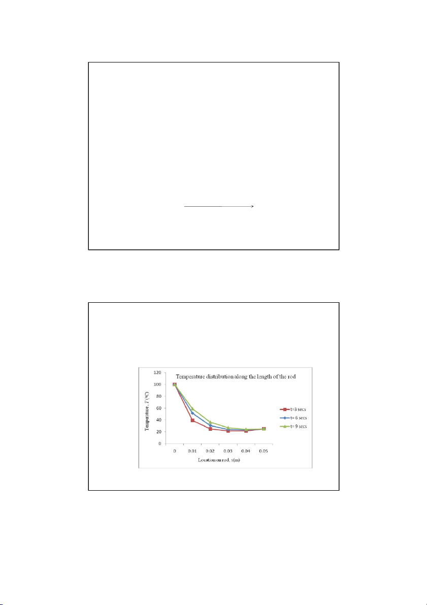
To better visualize the temperature variation at different
locations at different times, the temperature distribution along
the length of the rod at different times is plotted below. Son Dao, PhD © 30 30 15 12/16/2021 The Crank-Nicolson Method WHY: 2  T
Using the implicit method our approximation of was of 2 O(x) 2 x  
accuracy, while our approximation of T was of O (  t ) accuracy. t  Son Dao, PhD © 31 31 The Crank-Nicolson Method
One can achieve similar orders of accuracy by approximating the
second derivative, on the left hand side of the heat equation, at the
midpoint of the time step. Doing so yields 2T   j j j j 1 j 1 j 1 T  2T   T T 2T T i 1 i  i 1        i i i 2   1 1 x 2 x x i, j   2  2   Son Dao, PhD © 32 32 16 12/16/2021 The Crank-Nicolson Method
The first derivative, on the right hand side of the heat equation, is
approximated using the forward divided difference method at time level j  1 , T T j1  T j i i  t t i , j Son Dao, PhD © 33 33 The Crank-Nicolson Method
•Substituting these approximations into the governing equation for heat conductance yields    1  1  T j  1 1  2 2 1 T j T j1 T j   T j  T j  1  T j  Tj i i i i i i 1 i i   2    2 2  x    x    t  giving j 1  j 1  j 1 j j j   T  2 1 (  ) T   T   T  2 1 (  ) T   T i 1  i i 1  i  1 i i  1 where t      2 x
•Having rewritten the equation in this form allows us to descritize
the physical problem. We then solve a system of simultaneous linear
equations to find the temperature at every node at any point in time. Son Dao, PhD © 34 34 17 12/16/2021 Example 3: Crank-Nicolson
Consider a steel rod that is subjected to a temperature of 1 0 0 C  on the left end and 2 5 C
 on the right end. If the rod is of length . 0 0 5 m ,use the Crank-
Nicolson method to find the temperature distribution in the rod from t  0 to t  9 seconds. Use  x  0 . 0 1 m ,  t  3 s. kg J Given:  54 W k ,   7 8 0 0 , C  490 m  K 3 m kg  K
The initial temperature of the rod is 2 0 C  . i  0 1 2 3 4 5 T 10  0 C T 25 C  0 0 . m 1 Son Dao, PhD © 35 35 Example 3: Crank-Nicolson Recall, Number of time steps, k t t   final initial  C  t 9 0 therefore,  3 54    7800  490 3.  4 . 1 129 10 5   m 2 / s. Boundary Conditions j T  100  C Then, 0 j  for all j  , 1 , 0 2 3 , t     T  C  5 25   2 x 3 5  1 4 . 129 10  All internal nodes are at 2 0 C  0.012 for t  0 s e c . This can be  0 4 . 239 . represented as, 0 T  20C, for a l li  1,2,3,4 i Son Dao, PhD © 36 36 18 12/16/2021 Example 3: Crank-Nicolson Nodal temperatures when t  0 se c , j  0: T 0  100 C  0 0 T  20 C 1  0 T  20 C 2 I  nterior n odes 0 T  20 C 3  0 T  20  C 4  T 0  25 C  5
We can now form our system of equations for the first time step by
writing the approximated heat conduction equation for each node. j 1 j  1 j  1 j j j  T               2 1 ( T ) T  T 2 1 ( T ) T i 1 i i 1 i 1  i i 1  Son Dao, PhD © 37 37 Example 3: Crank-Nicolson Nodal temperatures when t  3 se c , (Example Calculations) 1 i  0
T  100C  Boundary Condition 0
For the interior nodes setting j  0 and i , 1  , 2 , 3 4 gives the following i  1 1  T   2 1 (  ) 1 1 0 T  T   T   2 1 (  ) 0 0 T  T  0 1 2 0 1 2 ( . 0 4239 100)  2 1 (  0 4 . 239) 1 T  0 4 . 239 1 T  (0 4 . 239 1 ) 00  2 1 (  0 4 . 239)20  0 ( 4 . 239)20 1 2  42.39  2 8 . 478 1 T  0 4 . 239 1 T  42.39  23 0 . 44  8 4 . 78 1 2 . 2 8478 1 T  . 0 4239 1 T  116 3 . 0 1 2
For the first time step we can write four such equations with four
unknowns, expressing them in matrix form yields  . 2 8478  . 0 4239 0 0   T 1 11 . 6 30    1  1    . 0 4239 . 2 8478  . 0 4239 0   T2  4 . 0 000     0  . 0 4239 8 . 2 478  . 0 4239    1 T 4 . 0 000    3     0 0 0 4 . 239 . 2 8478 Son D   a T o, P   1 hD © 38 4 5 . 2 718 38 19 12/16/2021 Example 3: Crank-Nicolson  8 . 2 478  0 4 . 239 0 0   1 T  116 3 . 0     11    4 . 0 239 . 2 8478  . 0 4239 0  T2 4 . 0 000     0 0 4 . 239 . 2 8478  . 0 423  9  1   T 4 . 0 000     3  1    0 0  . 0 4239 .
2 8478  T4 5 . 2 718 
The above coefficient matrix is tri-diagonal. Special algorithms
such as Thomas’ algorithm can be used to solve simultaneous
linear equation with tri-diagonal coefficient matrices. The solution is given by  1 T   100  0  1 T  44 3 . 7  2  1    1 Hence, the nodal T 44.372   1    1   T 23 7 . 46  1  T  23.746 2 temps at t  3 s e c are      2       1 T 20 7 . 9  7  1 T3   20.797  3  1    1    T 21.607 T4  21 6 . 0  7  4     1 T    5   25  Son Dao, PhD © 39 39 Example 3: Crank-Nicolson Nodal temperatures when t  6 se c , (Example Calculations) 2 i  0
T  100C  Boundary Condition 0
For the interior nodes setting j  1and i , 1  , 2 , 3 4 gives the following, i  1 2  T   2 1 (  ) 2 2 1 T  T   T   1 ( 2  ) 1 1 T  T  0 1 2 0 1 2 ( 4 . 0 239 100)  1 ( 2  . 0 4239) 2 T  . 0 4239 2 T  1 2 ( 4 . 0 239 1 ) 00  2 1 (  0 4 . 23 ) 9 44.372  ( 4 . 0 23 ) 9 2 . 3 746  42.39 . 2 8478 2 T  T    1 0 4 . 239 22 42.39 51.125 10.066 2.8478 2 T  0 4 . 239 2 T  145.971 1 2
For the second time step we can write four such equations with four
unknowns, expressing them in matrix form yields  2 8 . 478 0 4 . 239 0 0   2 T  145 9 . 71    12     0 4 . 239 2 8 . 478  0 4 . 239 0  T2  54 9 . 85     0  0 4 . 239 2 8 . 478  0 4 . 23  9  2  T  43 1 . 87     3  2    0 0  0.4239 2 8 . 478 Son  D  a T o, PhD © 40 4    54 9 . 08  40 20 12/16/2021 Example 3: Crank-Nicolson  8 . 2 478  4 . 0 239 0 0  2 T  145 9 . 71   12     0 4 . 239 2 8 . 478  0 4 . 239 0  2 T  54 9 . 85     0  0 4 . 239 . 2 8478  . 0 4239  2  T 43 1 . 87    3  2    0 0  0 4 . 239 .
2 8478 T4  54 9 . 08 
The above coefficient matrix is tri-diagonal. Special algorithms
such as Thomas’ algorithm can be used to solve simultaneous
linear equation with tri-diagonal coefficient matrices. The solution is given by  2 T   100  0  2 T  55 8 . 83   2    1 Hence, the nodal T 55.883   1    2    T 31 0 . 75  2  T 31.075 2 temps at t  6 s e c are       2      2  T 23 1 . 74   2 T3  23.174  3   2  2    T 22.730 T 4 4   22 7 . 30       2 T    5   25  Son Dao, PhD © 41 41 Example 3: Crank-Nicolson Nodal temperatures when t  9 se c , (Example Calculations) 3 i  0
T  100C  Boundary Condition 0
For the interior nodes setting j  2 and i , 1  , 2 , 3 4 gives the following, i  1 3  T  1 ( 2   ) 3 3 2 T   T  T  1 ( 2   ) 2 2 T  T 0 1 2 0 1 2 ( 0  4 . 239 1  0 ) 0  1 ( 2 0.423 ) 9 3 T 0.4239 3 T  2 2 (0 4 . 239 1 ) 00  1 ( 2  0 4 . 23 ) 9 55 8 . 83  0 ( .4239)31 0 . 75  4 . 2 39 2.8478 3 T  0.4239 3 T  4 . 2 39  64 3 . 88  13 1 . 73 1 2 8 . 2 478 3 T  . 0 4239 3 T 1  6 . 2 34 1 2
For the third time step we can write four such equations with four
unknowns, expressing them in matrix form yields  . 2 8478  4 . 0 239 0 0   3 T  162 3 . 4    13     4 . 0 239 . 2 8478  . 0 4239 0  T2  6 . 9 31  8   0  4 . 0 239 8 . 2 478  . 0 423  9  3  T 4 . 9 50  9    3     0 0 0 4 . 239 . 2 8478  Son  3 T D 4 ao  , PhD  5 © . 7 21  0 42 42 21 12/16/2021 Example 3: Crank-Nicolson  2.8478  0 4 . 239 0 0   3 T  162 3 . 4     13     0 4 . 239 . 2 8478  0 4 . 239 0  T2  6 . 9 318    0  0 4 . 239 2 8 . 478  0.423  9  3  T 4 . 9 509     3  3    0 0  0 4 . 239 2 8
. 478  T4  5 . 7 210 
The above coefficient matrix is tri-diagonal. Special algorithms
such as Thomas’ algorithm can be used to solve simultaneous
linear equation with tri-diagonal coefficient matrices. The solution is given by  3 T  0  100   3 T  62 6 . 04  3   1 Hence, the nodal  T1  62.604 3    T 37 6 . 13 3 2 temps at t  9 s e c are      T  37.613   2   3  3   T 26 5 . 62 T 26.562  3   3    3   T  3   T 24.042 4   24 0 . 42  4     3 T   25   5    Son Dao, PhD © 43 43 Example 3: Crank-Nicolson
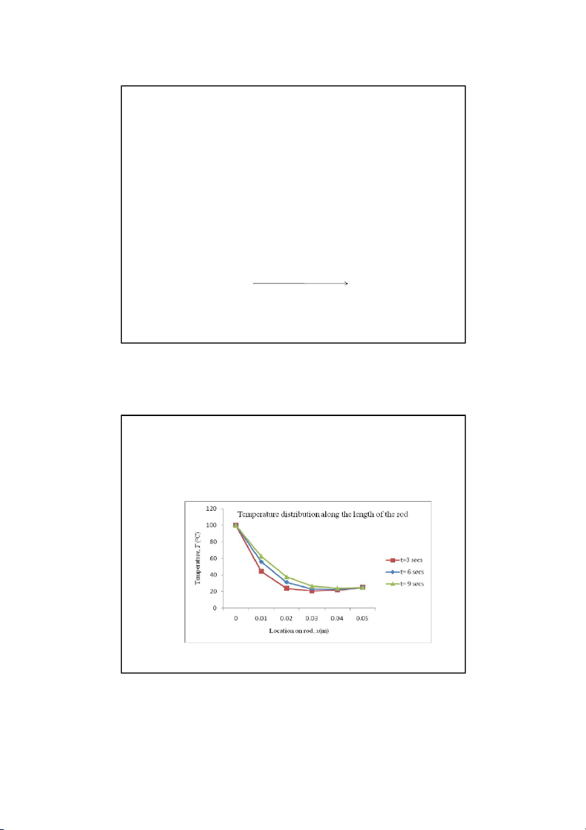
To better visualize the temperature variation at different
locations at different times, the temperature distribution along
the length of the rod at different times is plotted below. Son Dao, PhD © 44 44 22 12/16/2021
Internal Temperatures at 9 sec.
The table below allows you to compare the results from all three
methods discussed in juxtaposition with the analytical solution. Crank- Node Explicit Implicit Analytical Nicolson 3 T1 65 9 . 53 59 0 . 43 62 6 . 04 62 5 . 10 3 T 2 39 1 . 32 36 2 . 92 37 6 . 13 37 0 . 84 3 T3 27 2 . 66 26 8 . 09 26 5 . 62 25 8 . 44 3 T 4 22 8 . 72 24 2 . 43 24 0 . 42 23 6 . 10 Son Dao, PhD © 45 45 23