Multimedia data compression & coding: NFW final report môn Đa phương tiện và các ứng dụng giải trí | Trường Đại học Bách Khoa Hà Nội

HANOI UNIVERSITY OF SCIENCE AND TECHNOLOGY
---□&□--- ASSIGNMENT REPORT
TOPIC: NON-LINEAR FREQUENCY WARPING
Instructor
Assoc. Prof. Dr Phạm Văn Tiến Member Vũ Minh Hiển 20224311 Lê Hoàng Anh 20224297 Đào Hữu Mão 20233865 Phạm Thị Thanh Trúc 20224293 Subject
Multimedia data compression and coding Class 157320 Group 10 Table of Contents
I. Introduction ........................................................................................................... 3
II. Details .................................................................................................................. 4
2.1. Record the audio ........................................................................................... 4
2.2. Spectrum show and analysis ......................................................................... 4
2.2.1. Matlab coding .......................................................................................... 4
2.2.2. Spectrum analysis ................................................................................... 5
2.3. NFW Compression and Decompression ....................................................... 6
2.3.1. Audio Compression Using NFW .............................................................. 6
2.3.2. Audio Decompression Using NFW .......................................................... 7
Performance and Evaluation ............................................................................. 7
2.4. PSNR calculate and compare between NFW and MP3 ................................ 9
2.4.1. About PSNR ............................................................................................ 9
2.4.2. Convert .wav (original) file to .mp3 file .................................................... 9
2.4.3. Compare PNSR value of NFW codec and mp3 compression with original
.......................................................................................................................... 9
signal ................................................................................................................. 9
2.5. Generate MIDI music and perform a Jazz song .......................................... 12
III. CONCLUSION ..................................................................................................... 13
I. Introduction
- Students who have been contributing for the project: Vũ Minh Hiển
20224311 Creates a Jazz music mix, audio decompress.
Implemented the code for audio compress, decompress, Lê Hoàng Anh 20224297 PSNR comparation.
Convert .wav (original) file to .mp3 file, Calculate and Đào Hữu Mão 20233865 compare PSNR value.
Recording code, Spectrum Analysis, audio compress, Phạm Thị Thanh Trúc 20224293 report. - Brief view of the project:
This report provides a comprehensive overview of the process and outcomes of our
advanced audio coding project implemented using MATLAB. It outlines each stage
of the development in a clear, step-by-step manner, detailing the methods, algorithms,
and tools used throughout the project. The report also includes code snippets, visual
illustrations, and explanations to support and demonstrate our implementation. By
presenting both the theoretical background and practical execution, we aim to give
readers a complete understanding of how the project was carried out by our group.
II. Details 2.1. Record the audio
− Each of us recorded using phone, mix all with app and converted from mp3 to wav.
− We can also use the 'Part1_recording.m ' file to record
2.2. Spectrum show and analysis 2.2.1. Matlab coding
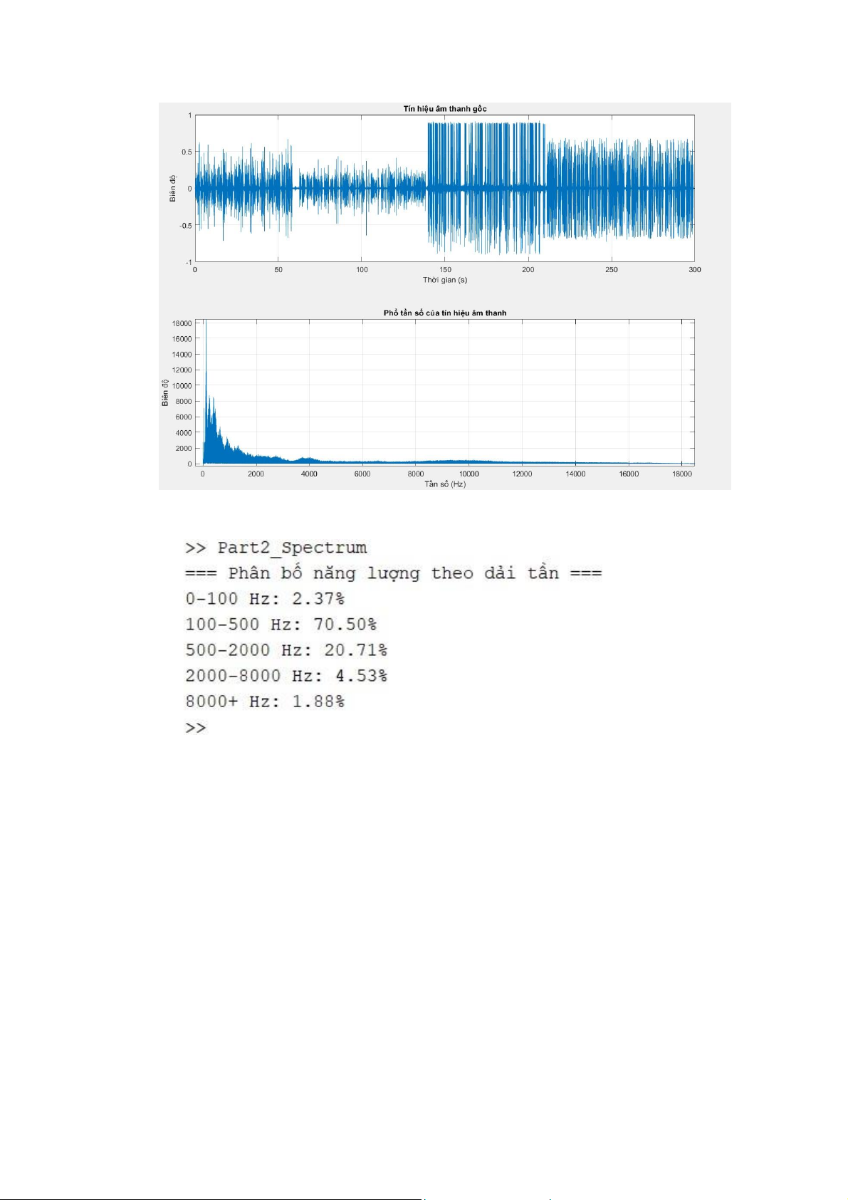
− After recording, our next task is using Matlab to show spectrum of the recorded audio
signal, then comments on its energy distribution over the frequency axis.
− This is the code we used and result: %% 1. Load Audio File
[y, fs] = audioread('recorded.wav'); y =
y(:,1); % Convert to mono if stereo %% 2. Spectrum Analysis % Calculate FFT N = length(y); Y = fft(y); f = linspace(0, fs, N); % Create figure with subplots
figure('Name', 'Audio Spectrum Analysis', 'Position', [100 100 1200 800]); % Plot 1: Time Domain Signal
subplot(2,1,1); t = (0:N-1)/fs;
plot(t, y); xlabel('Thời gian (s)'); ylabel('Biên độ');
title('Tín hiệu âm thanh gốc'); grid on; % Plot 2: Frequency Spectrum subplot(2,1,2);
plot(f(1:N/2), abs(Y(1:N/2)));
xlabel('Tần số (Hz)'); ylabel('Biên độ');
title('Phổ tần số của tín hiệu âm thanh'); grid on;
%% 3. Frequency Band Analysis % Define frequency bands
bands = [0 100; 100 500; 500 2000; 2000 8000; 8000 fs/2];
band_names = {'0-100 Hz', '100-500 Hz', '500-2000 Hz', '2000-8000 Hz', '8000+ Hz'};
energy_bands = zeros(length(bands), 1); % Calculate energy in each band
for i = 1:length(bands) band_indices = f >=
bands(i,1) & f <= bands(i,2); energy_bands(i) =
sum(abs(Y(band_indices)).^2); end % Normalize energy
energy_bands = energy_bands / sum(energy_bands) * 100; % Display energy distribution
disp('=== Phân bố năng lượng theo dải tần ==='); for i = 1:length(bands)
fprintf('%s: %.2f%%\n', band_names{i}, energy_bands(i)); end
− And it gives out the following result:
2.2.2. Spectrum analysis a. Frequency Band Analysis
− 0–100 Hz (2.37%): This very low-frequency range mostly contains background
noise, such as wind or unwanted ambient sounds.
− 100–500 Hz (70.50%): This range holds the majority of the signal’s energy. It likely
represents core sound components such as human speech fundamentals or main
musical tones, making it a crucial frequency band for natural audio.
− 500–2000 Hz (20.71%): This band contains clearer, more detailed audio
components — often speech formants or instrumental harmonics that enhance clarity.
− 2000–8000 Hz (4.53%): Higher-frequency components contributing to brightness or
timbral nuance, usually from vocals or high-pitched instruments. These are
perceptually important but lower in energy.
− 8000+ Hz (1.88%): This ultrasonic range contains very little energy and likely holds
inaudible frequencies or minor noise, often non-essential for perceptual audio quality. b. Observations
− The energy distribution reflects the nature and quality of the recorded audio. In the
case of speech, most energy resides in low to mid-frequency bands, which is consistent with the analysis.
− The dominance of the 100–500 Hz band indicates this is the primary region carrying meaningful audio content.
− Frequencies above 8000 Hz contribute little to the overall energy and may be safely
discarded or heavily compressed without noticeable quality loss.
c. Recommendation for Compression
Based on this analysis, we recommend prioritizing the preservation of low and
midfrequency bands during compression, while applying more aggressive reduction or
removal to high-frequency components. This strategy helps maintain perceptual quality
while significantly reducing file size.
2.3. NFW Compression and Decompression
2.3.1. Audio Compression Using NFW
Objective: The first script aims to compress an audio file using NFW, producing a .mat file
containing quantized magnitude and phase components.
Steps Involved:
1. Reading the Audio File:
a. The audio is read from a WAV file using audioread. The mono channel is selected for processing.
2. Short-Time Fourier Transform (STFT):
a. The audio signal is divided into frames using a windowed STFT process
(with a 2048-sample frame length and 1024-sample hop length).
b. FFT is applied to each frame to generate the STFT matrix, which contains
both magnitude and phase information for each frequency bin.
3. Non-linear Frequency Warping (Mel Scaling):
a. The frequency bins are warped using Mel scaling to mimic the human
auditory system's frequency perception.
b. The warped frequency indices are used to re-assign magnitudes from the
original STFT to a Mel-scaled matrix. 4. Quantization:
a. Both magnitude and phase matrices are quantized. Magnitudes are quantized
with 6 bits, and phase information is quantized with 4 bits. This reduces the
bit-depth, lowering the storage requirement.
5. Saving the Compressed Data:
a. The quantized magnitude and phase are stored in a .mat file, alongside the
parameters necessary for decompression (sampling frequency, frame length, hop length, etc.).
b. The compression ratio is calculated, comparing the original and compressed bit sizes. Output:
• A .mat file containing the compressed magnitude and phase data.
Compression Information: The script prints the compression ratio, original file size, and
compressed file size for transparency.
2.3.2. Audio Decompression Using NFW
Objective: The second script reconstructs the audio from the compressed .mat file,
reversing the NFW process and producing a reconstructed audio file in .wav format.
Steps Involved:
1. Loading the Compressed Data:
a. The compressed file is loaded to extract the quantized magnitude and phase,
as well as the original audio parameters (frame length, hop length, etc.). 2. Dequantization:
a. The magnitude and phase values are dequantized, reversing the quantization
process by mapping back the levels to the original range.
3. Inverse Frequency Warping (De-warping):
a. The Mel-scaled magnitude and phase are mapped back to the linear
frequency scale. This involves interpolating between the warped indices to
reconstruct the original frequency bins.
4. Reconstruction of the Full Spectrum:
a. The full spectrum (both positive and negative frequencies) is reconstructed
by applying conjugate symmetry for real signals.
5. Inverse Short-Time Fourier Transform (ISTFT):
a. The inverse STFT is applied using the Overlap-Add method. The frames are
synthesized from the magnitude and phase information and combined to
produce the time-domain signal.
6. Saving the Decompressed Audio:
a. The decompressed audio is saved as a .wav file, normalized to prevent
clipping, and played back to compare with the original audio. Output:
• A .wav file containing the decompressed audio.
Decompression Information:
• The script prints details such as the input and output file names, sampling frequency, and audio duration.
Performance and Evaluation Compression Ratio:
• The compression ratio is an important metric. The original audio file is typically in
16-bit PCM format, while the compressed version uses 6-bit magnitude and 4-bit
phase, significantly reducing the storage size. Quality Assessment:
• The decompressed audio is played back and compared with the original to evaluate
the perceptual quality. Since this is a lossy compression method, there might be
some degradation in quality, but the compression ratio and file size reduction justify
its use in storage-limited applications.
2.4. PSNR calculate and compare between NFW and MP3 2.4.1. About PSNR
- PSNR (Peak Signal-to-Noise Ratio) measures the reconstruction quality of a signal
after processing (such as compression and decompression) compared to the original
signal. In the context of audio
• Original signal: recorded.wav (the original audio).
• Reconstructed signal: compressed_mel.wav (the audio after compression and decompression).
- PSNR calculates the error between the two signals in the same domain (either time
or frequency), typically in the time domain (i.e., WAV audio samples).
2.4.2. Convert .wav (original) file to .mp3 file
1. Install FFmpeg for Windows
1. Go to: https://ffmpeg.org/download.html
2. Choose Windows → follow the link to gyan.dev.
3. Download ffmpeg-master-latest-win64-gpl.zi.
4. Extract and add the path of bin folder to your Windows PATH.
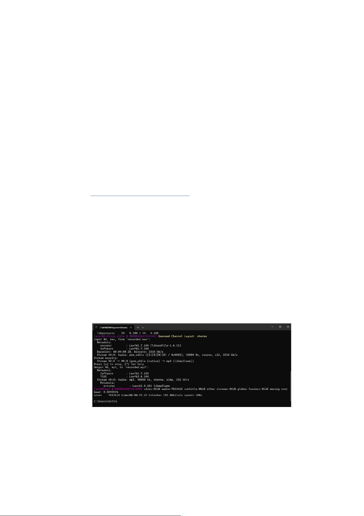
2. Use FFmpeg to convert .wav file to .mp3 file 1. Open terminal.
2. Check ffmpeg --version.
3. Copy .wav file to C:\Users\Dell (your path). 4. In terminal, enter:
ffmpeg -i recorded.wav -codec:a libmp3lame -b:a 192k recorded.mp3 The final screen should be:
Then check C:\Users\Dell (your path) again to get .mp3 file.
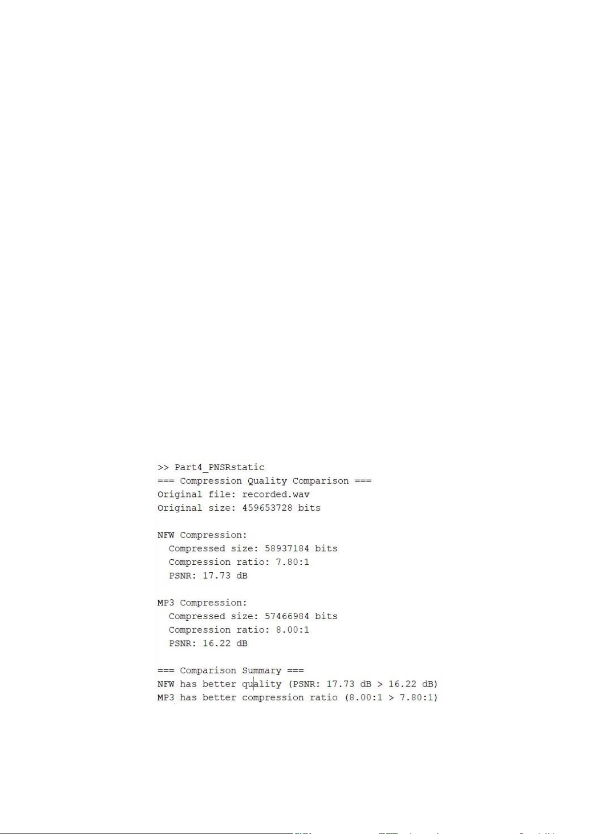
2.4.3. Compare PNSR value of NFW codec and mp3 compression with original signal
- On the next section of the assignment, we had to calculate the PSNR using this code: input_file = 'recorded.wav';
compare_compression_quality(input_file);
function compare_compression_quality(input_file) try %% 1. Load Original Audio
[original, fs] = audioread(input_file);
original = original(:,1); % Convert to mono if stereo
%% 2. Load NFW Compressed Audio % Load decompressed NFW audio
decompressed_nfw_file = 'decompressed.wav';
if ~exist(decompressed_nfw_file, 'file')
error('File giải nén NFW không tồn tại. Vui lòng chạy hàm decompress_NFW trước.'); end
[nfw_audio, ~] = audioread(decompressed_nfw_file); nfw_audio
= nfw_audio(:,1); % Convert to mono if stereo %% 3. Load MP3 Audio % Load MP3 audio mp3_file = 'recorded.mp3';
[mp3_audio, ~] = audioread(mp3_file); mp3_audio =
mp3_audio(:,1); % Convert to mono if stereo %% 4.
Ensure All Audio Signals Have Same Length
min_length = min([length(original), length(nfw_audio), length(mp3_audio)]);
original = original(1:min_length); nfw_audio = nfw_audio(1:min_length);
mp3_audio = mp3_audio(1:min_length); %% 5. Calculate PSNR % Calculate PSNR for NFW
nfw_mse = mean((original - nfw_audio).^2);
if nfw_mse == 0 nfw_psnr = Inf; else
nfw_psnr = 10 * log10(1 / nfw_mse); end % Calculate PSNR for MP3
mp3_mse = mean((original - mp3_audio).^2);
if mp3_mse == 0 mp3_psnr = Inf; else
mp3_psnr = 10 * log10(1 / mp3_mse); end
%% 6. Calculate Compression Ratios
% Original file size original_info = dir(input_file);
original_size = original_info.bytes * 8; % Convert to bits % NFW compressed size
compressed_nfw_file = 'compressed.mat'; if
~exist(compressed_nfw_file, 'file')
error('File nén NFW không tồn tại. Vui lòng chạy hàm compress_NFW trước.'); end
nfw_info = dir(compressed_nfw_file); nfw_size =
nfw_info.bytes * 8; % Convert to bits nfw_ratio = original_size / nfw_size;
% MP3 compressed size mp3_info = dir(mp3_file);
mp3_size = mp3_info.bytes * 8; % Convert to bits
mp3_ratio = original_size / mp3_size; %% 7. Display Results
fprintf('=== Compression Quality Comparison ===\n');
fprintf('Original file: %s\n', input_file); fprintf('Original
size: %d bits\n', original_size); fprintf('\n');
fprintf('NFW Compression:\n'); fprintf(' Compressed
size: %d bits\n', nfw_size); fprintf(' Compression
ratio: %.2f:1\n', nfw_ratio); fprintf(' PSNR: %.2f
dB\n', nfw_psnr); fprintf('\n');
fprintf('MP3 Compression:\n'); fprintf(' Compressed
size: %d bits\n', mp3_size); fprintf(' Compression
ratio: %.2f:1\n', mp3_ratio); fprintf(' PSNR: %.2f dB\n', mp3_psnr); % So sánh kết quả
fprintf('\n=== Comparison Summary ===\n'); if nfw_psnr > mp3_psnr
fprintf('NFW has better quality (PSNR: %.2f dB > %.2f dB)\n', nfw_psnr, mp3_psnr); elseif mp3_psnr > nfw_psnr
fprintf('MP3 has better quality (PSNR: %.2f dB > %.2f dB)\n', mp3_psnr, nfw_psnr); else
fprintf('Both methods have the same quality (PSNR: %.2f dB)\n', nfw_psnr); end if nfw_ratio > mp3_ratio
fprintf('NFW has better compression ratio (%.2f:1 > %.2f:1)\n', nfw_ratio, mp3_ratio);
elseif mp3_ratio > nfw_ratio
fprintf('MP3 has better compression ratio (%.2f:1 > %.2f:1)\n', mp3_ratio, nfw_ratio); else
fprintf('Both methods have the same compression ratio (%.2f:1)\n', nfw_ratio); end %% 8. Visual Comparison % Create time-domain plots figure; subplot(3,1,1); plot(original); title('Original Audio'); xlabel('Sample'); ylabel('Amplitude'); subplot(3,1,2); plot(nfw_audio); title('NFW Compressed Audio'); xlabel('Sample'); ylabel('Amplitude'); subplot(3,1,3); plot(mp3_audio); title('MP3 Compressed Audio'); xlabel('Sample'); ylabel('Amplitude');
% Create frequency-domain plots figure;
subplot(3,1,1); plot_spectrum(original,
fs); title('Original Audio Spectrum'); subplot(3,1,2); plot_spectrum(nfw_audio, fs);
title('NFW Compressed Audio Spectrum'); subplot(3,1,3); plot_spectrum(mp3_audio, fs);
title('MP3 Compressed Audio Spectrum'); % Create error plots figure; subplot(2,1,1); plot(original - nfw_audio); title('Error: Original - NFW'); xlabel('Sample'); ylabel('Amplitude'); subplot(2,1,2); plot(original - mp3_audio); title('Error: Original - MP3'); xlabel('Sample'); ylabel('Amplitude'); %% 9. Play Audio for Comparison disp('Playing original audio...'); sound(original, fs); pause(length(original) /fs + 1); disp('Playing NFW compressed audio...'); sound(nfw_audio, fs); pause(length(nfw_audio )/fs + 1); disp('Playing MP3 compressed audio...'); sound(mp3_audio, fs); catch ME
fprintf('Error in comparison: %s\n', ME.message);
fprintf('Stack trace:\n'); disp(ME.stack);
rethrow(ME); end end function plot_spectrum(x, fs) % Calculate spectrum N = length(x); X = fft(x); f = linspace(0, fs/2, N/2+1); % Plot magnitude spectrum plot(f, 2*abs(X(1:N/2+1))/N); xlabel('Frequency (Hz)'); ylabel('Magnitude'); xlim([0 min(20000, fs/2)]); end - The result show that:
2.5. Generate MIDI music and perform a Jazz song
− Here is the code to generate midi background music in Python:
from mido import Message, MidiFile, MidiTrack import random
# Tổng thời gian mong muốn: 5 phút = 300 giây
# Với tempo mặc định: 500000 us/beat = 0.5s/beat
# 480 ticks per beat (default) # => 1 giây = 960 ticks
# => 5 phút = 300 giây = 288000 ticks
total_ticks = 288000 ticks_per_note = 600 num_notes
= total_ticks // ticks_per_note # => 480 nốt mid = MidiFile() track = MidiTrack() mid.tracks.append(track)
track.append(Message('program_change', program=0, time=0)) for i in range(num_notes):
note = random.choice([60, 62, 65, 67, 69, 72])
velocity = random.randint(60, 90)
track.append(Message('note_on', note=note, velocity=velocity, time=200))
track.append(Message('note_off', note=note, velocity=0, time=400)) mid.save('midi_output.mid')
- The last thing we do: combining recorded audio and backgroun audio .wav( that is
transfered from the midi ouput generated from the python file.
[y1, fs1] = audioread('recorded.wav');
[y2, fs2] = audioread('midi_output.wav');
% Chuyển về mono nếu cần if size(y1,2) > 1 y1 = mean(y1, 2); end if size(y2,2) > 1 y2 = mean(y2, 2); end
% Cắt đến độ dài nhỏ nhất min_len =
min(length(y1), length(y2)); y1 =
y1(1:min_len); y2 = y2(1:min_len);
% Mix với hệ số 0.5 để tránh clipping mixed = y1 + 0.5 * y2;
mixed = mixed / max(abs(mixed)); % Chuẩn hóa
audiowrite('jazz_mix.wav', mixed, fs1); fprintf("✅
Đã tạo thành công jazz_mix.wav\n"); III. CONCLUSION
This is our first big assignment regarding the Multimedia Data Compression And Coding
subject. Albeit very amateur on working on all problems, it is also such a essential
objective for us – not only a student of Hust but also a member of ET-E16 major to gain
a plethora of experiences in terms of both knowledge and cooperation, aiming for further education in multimedia.
In this project, we successfully applied Non-linear Frequency Warping (NFW)
combined with quantization to compress audio signals efficiently. The analysis of
frequency energy distribution helped us focus on preserving essential low- and
midfrequency components while discarding high-frequency details that contribute less to perceived quality.
Additionally, we generated a MIDI jazz sequence using a randomized C major jazz
scale. This showcased how programmatic music creation can be used to simulate
realistic audio with minimal file size, suitable for embedded or multimedia systems.
Overall, both the compression technique and MIDI synthesis demonstrated effective
strategies for audio size reduction and generation without sacrificing perceptual quality.