Scheduling problem - schedule orders to minimize the total cost of delay in production systems | Báo cáo học phần Deterministic Models in Operations Research | Trường Đại học Quốc tế, Đại học Quốc gia Thành phố Hồ Chí Minh

In Vietnam, manufacturing plants that manage extensive operations that require assigning people and resources to tasks at specific times must regularly address complex scheduling issues. Scheduling is a manufacturing process that involves performing many tasks on a limited set of machines, each of which can perform only one task at a time. One common scheduling problem is a job shop concerns the scheduling of tasks on production lines or in warehouse halls. The job-shop problem is the most general and universal of scheduling problems. It assumes a complete order of tasks and operations and adopts specific guidelines and limitations resulting from technology (e.g. no machine can perform more than one operation at the same time). The problem consists in determining the optimal solution that will reduce the resources involved (time, machines, employees) for performing all operations of the considered process. Tài liệu giúp bạn tham khảo, ôn tập và đạt kết quả cao. Mời bạn đón xem.

International University – VNUHCM Deterministic Models in Operation Research School
of Industrial Engineering and Management Year: 2022-2023
1
INTERNATIONAL UNIVERSITY
VIETNAM NATIONAL UNIVERSITY - HO CHI MINH CITY
SCHOOL OF INDUSTRIAL ENGINEERING AND MANAGEMENT
PROJECT REPORT
Deterministic Models in Operations Research _ G01
Topic: Scheduling problem - schedule orders to minimize the total cost of delay in
production systems _ Group 09
No.
FULL NAME
STUDENT ID
CONTRIBUTION
1
Nguyễn Thị Phương Anh
IELSIU21006
100%
2
Dương Nguyễn Cát Tường
IELSIU 21171
100%
3
Lê Thị Thu Hà
IELSIU21194
100%
4
Lê Thị Huỳnh Mai
IELSIU21116
100%
5
Lê Ngọc Y Khánh
IELSIU21207
100%
lOMoARcPSD|4720736International University – VNUHCM Deterministic Models in Operation Research School
of Industrial Engineering and Management Year: 2022-2023
TABLE OF CONTENTS
2
I. INTRODUCTION .................................................................................................. 5
1. Background of Study: ............................................................................................. 5
2. Problem Statement .................................................................................................. 5
3. Objectives ............................................................................................................... 6
4. Scope and Limitations............................................................................................. 6
II. MATHEMATICAL MODEL/ ALGORITHMS ................................................. 7
1. Parameters ............................................................................................................... 7
2. Decision Variables................................................................................................... 7
3. Objective Function .................................................................................................. 8
4. Constraints .............................................................................................................. 8
III. RESULT ANALYSIS AND DISCUSSION ........................................................ 9
1. Processing and Result Analysis .............................................................................. 9
2. Sensitivity Analysis ............................................................................................... 11
3. Solution Discussion .............................................................................................. 16
4. Future Development .............................................................................................. 17
IV. CONCLUSION ................................................................................................... 18
V. REFERENCES ..................................................................................................... 18
VI. APPENDIX ......................................................................................................... 18
1. CPLEX code ......................................................................................................... 18
2. Data Input .............................................................................................................. 20
3. Output data from Cplex: ....................................................................................... 25
Table 1: The table when changing available date of resource by 2 units .....................
12
Table 2: The data input when decreasing contract value by 1% .................................. 14
Table 3: The data input when decreasing contract value by 2% .................................. 15
Table 4: Customer order ............................................................................................... 20
Table 5: Unit processing time (day) ............................................................................. 21
International University – VNUHCM Deterministic Models in Operation Research School
of Industrial Engineering and Management Year: 2022-2023
TABLE OF CONTENTS
3
Table 6: Order division ................................................................................................. 21
Table 7: Cost of order delay ......................................................................................... 23
lOMoARcPSD|4720736International University – VNUHCM Deterministic Models in Operation Research School
of Industrial Engineering and Management Year: 2022-2023
TABLE OF CONTENTS
4
Figure 1: Solution from the code (1) .............................................................................. 9
Figure 2: The statistics of the solution ......................................................................... 10
Figure 3: The value for Z .............................................................................................. 10
Figure 4: Solution from the code (2) ............................................................................ 24
International University – VNUHCM Deterministic Models in Operation Research School
of Industrial Engineering and Management Year: 2022-2023
5
I. INTRODUCTION
1. Background of Study:
Operations Research (OR) is the advanced scientific method to help make better
choices in supply chain management. This is an analytical problem-solving and
decision-making technique useful in managing organizations. In operations
research, problems are broken down into their basic components and then solved
in specific steps using mathematical analysis.
In Vietnam, manufacturing plants that manage extensive operations that require
assigning people and resources to tasks at specific times must regularly address
complex scheduling issues. Scheduling is a manufacturing process that involves
performing many tasks on a limited set of machines, each of which can perform
only one task at a time. One common scheduling problem is a job shop concerns
the scheduling of tasks on production lines or in warehouse halls. The job-shop
problem is the most general and universal of scheduling problems. It assumes a
complete order of tasks and operations and adopts specific guidelines and
limitations resulting from technology (e.g. no machine can perform more than
one operation at the same time). The problem consists in determining the optimal
solution that will reduce the resources involved (time, machines, employees) for
performing all operations of the considered process.
The goal of the job shop problem is to minimize the time interval: the time
interval from the earliest job start time to the latest finish time. Each job consists
of a sequence of tasks that must be executed in a specified order, and each task
must be processed on a specific machine. The problem is to schedule the tasks on
the machines in such a way as to minimize the length of the schedule - the time
required to complete all the tasks.
We apply operations research to the job shop problem to optimize the cost of
operation by influencing the tardiness and lateness of each stage of the production
process.
2. Problem Statement
There are still scheduling issues that prevent Vietnam from having an efficient
method for producing wooden products. In this project, our team will provide an
International University – VNUHCM Deterministic Models in Operation Research School
of Industrial Engineering and Management Year: 2022-2023
6
order allocation and integer programming approach to production scheduling to
solve the potential delays and lateness that affect the production process from the
perspective of make-to-order manufacturing. We assume that our company has a
total of 28 products such as bed, table, chair, cabinet,...with different data.
Applying some restrictions to see how tardiness and lateness would be influenced
led to the cost of operation being optimized.
3. Objectives
According to the information given above, we have two core objectives for this
case:
Objective 1: Minimizing the cost of operation due to tardiness.
Objective 2: Minimizing the tardiness of each process.
Moreover, the primary goal of our report's CPLEX model is to have a benchmark
for algorithms, hence, the model in our report can only resolve parts of the
objectives above.
4. Scope and Limitations
1.4.1 Scope:
This project focuses on applying integer linear programming and building the
CPLEX model that can minimize the total tardiness of our Company. In this
model, a group of customer orders are first arranged to be completed, and then
without any intermediary inventory, they are sent directly to the customers.
Finding a combined production and distribution plan that will maximize both
customer satisfaction and overall distribution costs is the aim. In the study, a
mixed integer program was suggested as a use for long-term production schedules
in make-to-order manufacturing to determine the ideal value of the maximum
earliness.
1.4.2 Limitations:
Although our model could make a result and reach the standard target our group
expected at the beginning of the project, there still have some limitations in
practical application.
International University – VNUHCM Deterministic Models in Operation Research School
of Industrial Engineering and Management Year: 2022-2023
7
Firstly, due to the limited information about the database published, we can use
this model, we decided to create available data based on relevant information.
Additionally, as we create the database, we can only force the model to run with
limited data to avoid as many inconsistent errors as if we run this model with
unlimited data.
Secondly, the data we selected is the default information at the same time in the
past, and we built the model to improve the profit of the company. However, for
that reason, this model can not be used immediately if we do not know how many
orders and the quantity of each order. Moreover, if the list of orders is
continuously adjusted will make the accuration of calculating the minimization
of tardiness diminished.
Lastly, the model is for the constant process which means there is no interruption
such as broken machines, laid off,...
II. MATHEMATICAL MODEL/ ALGORITHMS
1. Parameters
Notations i: the order i t:
the time period t (day) Set:
O: set of order
O1Set: set of small batches
O2Set: set of large batches
T: set of planning periods
Parameters:
d
i
: due date of order i
P
i
: processing time of one unit of each order
N: the limit of processing time in one day
A
i
: available date of material of each order
C
i
: the cost of tardiness of each order
2. Decision Variables
X
it
: binary variable that indicates whether order i is performed in period t
International University – VNUHCM Deterministic Models in Operation Research School
of Industrial Engineering and Management Year: 2022-2023
8
Y
it
: fraction of order i to be processed in period t
Z
i
: binary variable that indicates whether order i is completed after due date TCD:
the total cost of delay
3. Objective Function
𝑂
𝑀𝑖𝑛𝑖𝑚𝑖𝑧𝑒 𝑇𝐶𝐷 = ∑ 𝑍
𝑖
∗ 𝐶
𝑖
𝑖
This objective function is to minimize the total cost of delay value.
4. Constraints
𝑇
𝑋
𝑖𝑡
= 1 𝑓𝑜𝑟 𝑎𝑙𝑙 𝑖 𝑂1𝑆𝑒𝑡, 𝑡 𝐴
𝑖
(1)
𝑡
𝑇−1
𝑋
𝑖𝑡
= 1 𝑓𝑜𝑟 𝑎𝑙𝑙 𝑖 𝑂2𝑆𝑒𝑡, 𝑡 𝐴
𝑖
(2)
𝑡
𝑋
𝑖𝑡
= 𝑌
𝑖𝑡
𝑓𝑜𝑟 𝑎𝑙𝑙 𝑖 𝑂1𝑆𝑒𝑡, 𝑡 𝑇 , 𝑡 𝐴
𝑖
(3)
𝐼𝑓 𝑋
𝑖𝑡
= 1 𝑡ℎ𝑒𝑛 𝑌
𝑖𝑡
≥ 0.3 ∗ 𝑋
𝑖𝑡
𝑎𝑛𝑑 𝑌
𝑖𝑡
+ 𝑌
𝑖(𝑡+1)
= 1
𝑓𝑜𝑟 𝑎𝑙𝑙 𝑖 𝑂2𝑆𝑒𝑡, 𝑡 ∈ (𝑇 − 1), 𝑡 𝐴
𝑖
(4)
𝑇
𝑍
𝑖
= ∑
𝑡
𝑋
𝑖𝑡
𝑓𝑜𝑟 𝑎𝑙𝑙 𝑖 𝑂1𝑆𝑒𝑡, 𝑡 𝑇 , 𝑡 > 𝑑
𝑖
(5)
𝑇
𝑍
𝑖
= ∑
𝑋
𝑖𝑡
𝑓𝑜𝑟 𝑎𝑙𝑙 𝑖 𝑂2𝑆𝑒𝑡, 𝑡 ∈ (𝑇 − 1), 𝑡 ≥ (𝑑
𝑖
− 1) (6)
𝑡
𝑂
𝑃
𝑖
∗ 𝑌
𝑖𝑡
𝑁 𝑓𝑜𝑟 𝑎𝑙𝑙 𝑖 𝑂, 𝑡 𝑇 (7)
𝑖
Explanation
International University – VNUHCM Deterministic Models in Operation Research School
of Industrial Engineering and Management Year: 2022-2023
9
- Constraints (1) and (2) are the order assignment of O1 set and O2 set.
- Constraints (3) ensures that each indivisible order is finished in one day.
- Constraints (4) ensures each divisible order is allocated among all the periods
according to its assignment.
- Constraints (5) indicates the indivisible tardy order is finished after its due date.
- Constraints (6) indicates the divisible tardy order is partly assigned after its due
date.
- Constraints (7) ensures the production time on one day cannot be over the
maximum available time on that day.
III. RESULT ANALYSIS AND DISCUSSION
1. Processing and Result Analysis
1.1 Output data from Cplex:
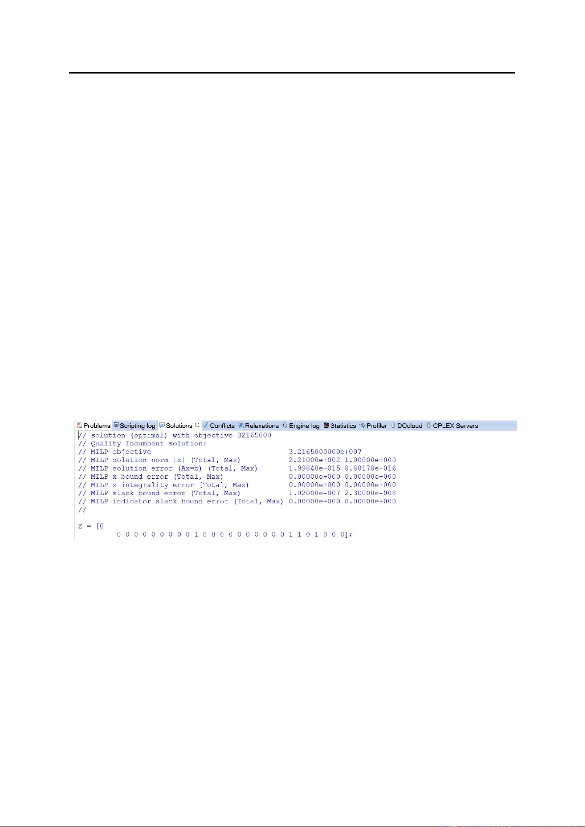
Figure 1: Solution from the code (1)
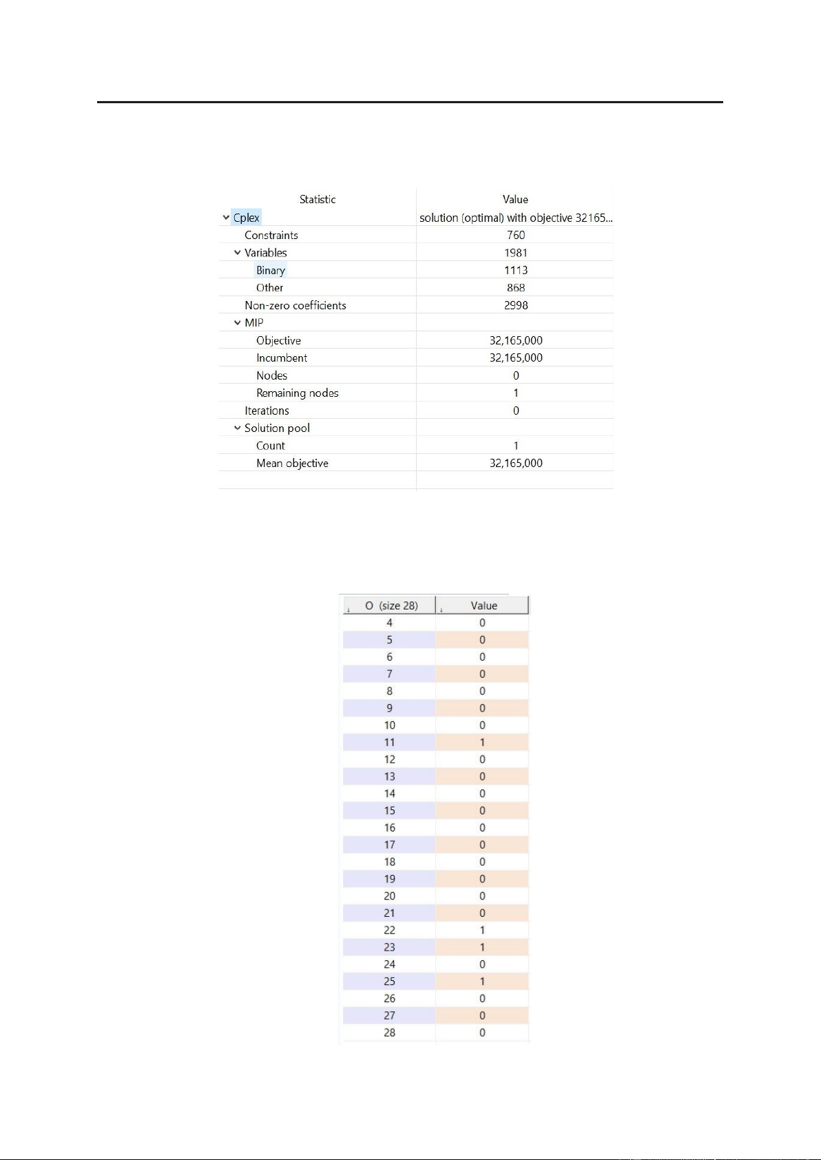
And the statistics of the solution above are shown following:
International University – VNUHCM Deterministic Models in Operation Research School
of Industrial Engineering and Management Year: 2022-2023
10
Figure 2: The statistics of the solution
1.2 Result analysis
International University – VNUHCM Deterministic Models in Operation Research School
of Industrial Engineering and Management Year: 2022-2023
11
Figure 3: The value for Z
After running this model, the number of tardy orders is 4, belonging to order numbers
11, 22, 23, and 25. Meanwhile, the code was able to find an optimal solution with an
objective value of 32165000 for a production line with 28 orders. The quality of the
solution was good, as evidenced by the low norm and error values. This suggests that
the code can find good solutions to MILP problems in the context of production line
scheduling.
2. Sensitivity Analysis
2.1. Case 1: Decreasing time period
In this case, we decrease the time period by 3 units from 31 to 28. After decreasing, we
obtain the result with the optimal solution is 4 delays which is order 11, 22, 23, 25 and
the objective value is 32165000
Z = [0 0 0 0 0 0 0 0 0 0 1 0 0 0 0 0 0 0 0 0 0 1 1 0 1 0 0 0];
2.2. Case 2: Decreasing available date
In this case, we decrease the available date of resource by 2 units if the available date is
more than 5 days. Then we have the input data is:
Order
Due date (day)
Available date of resource (day)
1
25
1
2
23
8
3
23
20
4
25
7
5
25
6
6
23
5
International University – VNUHCM Deterministic Models in Operation Research School
of Industrial Engineering and Management Year: 2022-2023
12
7
25
10
8
23
20
9
23
20
10
25
7
11
21
20
12
26
8
13
21
5
14
26
5
15
25
1
16
23
5
17
25
5
18
21
17
19
21
13
20
26
22
21
21
17
22
23
21
23
23
20
24
21
6
25
25
22
26
21
4
27
24
1
28
23
6
International University – VNUHCM Deterministic Models in Operation Research School
of Industrial Engineering and Management Year: 2022-2023
13
Table 1: The table when changing available date of resource by 2 units
After decreasing, we obtain the result with the optimal solution is 2 delays which is order
8, 11 and the objective value is 375000
Z = [0 0 0 0 0 0 0 1 0 0 1 0 0 0 0 0 0 0 0 0 0 0 0 0 0 0 0 0];
2.3. Case 3: Decreasing limit processing time
In this case, we decrease the limit processing time for 3 units from 16 to 13. After
decreasing, we obtain the result with the optimal solution is 4 delays which is order 11,
22, 23, 25 and the objective value is 32165000
Z = [0 0 0 0 0 0 0 0 0 0 1 0 0 0 0 0 0 0 0 0 0 1 1 0 1 0 0 0];
2.4. Case 4: Decreasing cost in contract
2.4.1. Decrease by 1%
In this case, we decrease 1% of the cost in contract. Then we have the input data is:
Order
Quantity
Price
Price of contract
Contract value (VND)
1
5
2500000
12500000
12375000
2
10
1200000
12000000
1188000
3
10
850000
8500000
841500
4
5
200000
1000000
99000
5
5
450000
2250000
2227500
6
10
1800000
18000000
1782000
7
5
400000
2000000
198000
International University – VNUHCM Deterministic Models in Operation Research School
of Industrial Engineering and Management Year: 2022-2023
14
8
15
190000
2850000
282150
9
10
500000
5000000
495000
10
10
230000
2300000
2277000
11
5
180000
900000
89100
12
5
250000
1250000
123750
13
15
150000
2250000
222750
14
12
700000
8400000
8316000
15
15
130000
1950000
193050
16
8
70000
560000
55440
17
10
250000
2500000
247500
18
10
50000
500000
49500
19
10
1300000
13000000
1287000
20
15
300000
4500000
4455000
21
20
2400000
48000000
4752000
22
20
1400000
28000000
27720000
23
15
1450000
21750000
2153250
24
25
1200000
30000000
2970000
25
20
950000
19000000
1881000
26
25
800000
20000000
1980000
27
30
1300000
39000000
3861000
28
25
1100000
27500000
27225000
Table 2: The data input when decreasing contract value by 1%
International University – VNUHCM Deterministic Models in Operation Research School
of Industrial Engineering and Management Year: 2022-2023
15
After decreasing, we obtain the result with the optimal solution is 4 delays which is order
11, 22, 23, 25 and the objective value is 31843350
Z = [0 0 0 0 0 0 0 0 0 0 1 0 0 0 0 0 0 0 0 0 0 1 1 0 1 0 0 0];
2.4.2. Decrease by 2%
In this case, we decrease 2% of the cost in contract. Then we have the input data is:
Order
Quantity
Price
Price of contract
Contract value (VND)
1
5
2500000
12500000
12250000
2
10
1200000
12000000
1176000
3
10
850000
8500000
833000
4
5
200000
1000000
98000
5
5
450000
2250000
2205000
6
10
1800000
18000000
1764000
7
5
400000
2000000
196000
8
15
190000
2850000
279300
9
10
500000
5000000
490000
10
10
230000
2300000
2254000
11
5
180000
900000
88200
12
5
250000
1250000
122500
13
15
150000
2250000
220500
14
12
700000
8400000
8232000
15
15
130000
1950000
191100
16
8
70000
560000
54880
17
10
250000
2500000
245000
International University – VNUHCM Deterministic Models in Operation Research School
of Industrial Engineering and Management Year: 2022-2023
16
18
10
50000
500000
49000
19
10
1300000
13000000
1274000
20
15
300000
4500000
4410000
21
20
2400000
48000000
4704000
22
20
1400000
28000000
27440000
23
15
1450000
21750000
2131500
24
25
1200000
30000000
2940000
25
20
950000
19000000
1862000
26
25
800000
20000000
1960000
27
30
1300000
39000000
3822000
28
25
1100000
27500000
26950000
Table 3: The data input when decreasing contract value by 2%
After decreasing, we obtain the result with the optimal solution is 4 delays
which is order 11, 22, 23, 25 and the objective value is 31521700
Z = [0 0 0 0 0 0 0 0 0 0 1 0 0 0 0 0 0 0 0 0 0 1 1 0 1 0 0 0];
3. Solution Discussion
3.1. Decreasing time period:
After reducing the time period by 3 units, the optimal value does not change, but
at least we can shorten the production time leading to the decreasing factory
operation cost and use time to produce other orders.
3.2. Decreasing available date:
International University – VNUHCM Deterministic Models in Operation Research School
of Industrial Engineering and Management Year: 2022-2023
17
It is clear that when we decrease the available date by 2 units if the available date
is more than 5 days then the optimal value reduces from 32 165 000 to 375 000
and the number of delays also reduces to 2 delays.
Therefore, if the company wants to reduce the available date in order to minimize
the cost due to tardiness, it is suggested that they should reduce 2 days for orders
that have more than 5 available days, then the optimal value will decrease by
98,8%.
3.3. Decreasing the processing time:
Same as the result of decreasing time period, after conducting a sensitivity
analysis on decreasing limit processing time by 3 units, the optimal value does
not change but it helps to reduce the production process that can optimize the
company's operating costs and take advantage of making other orders.
3.4. Decreasing cost in contract:
Obviously, The cost in contract is proportional to the optimal value, which means
the decreasing cost in contract leads to a reduction in the cost due to tardiness.
Simply, if the cost in contract decreases by 1% (from 335 460 000 to 109 346
490) and 2% (from 335 460 000 to 108 241 980) then the optimal value will also
decrease by the corresponding percentages of 31 843 350 and 31 521 700,
respectively.
4. Future Development
As the code continues to be developed, it has the potential to solve even larger
and more complex problems, including the automation of the scheduling process
entirely. By doing so, companies can free up valuable human resources to focus
on other critical tasks, such as research and development, which can ultimately
lead to further innovations and advancements in the industry.
Moreover, the project has the potential to improve the accuracy and reliability of
production scheduling, which can lead to increased customer satisfaction. With
precise scheduling and faster production times, companies can fulfill orders more
quickly and efficiently, reducing the risk of delayed deliveries or backlogs,
ultimately resulting in happier customers and improved business performance.
International University – VNUHCM Deterministic Models in Operation Research School
of Industrial Engineering and Management Year: 2022-2023
18
Overall, the sensitivity has the potential to transform the manufacturing industry,
optimizing production processes and allowing companies to remain competitive
in an ever-changing market. By leveraging this analysis, the company can
streamline its operations and achieve greater levels of success, paving the way
for a brighter and more efficient future.
IV. CONCLUSION
Originally, this project was applied to minimize the tardiness of each order and
then optimize the cost due to tardiness, which proposed a mixed-integer program
to use for long-term production schedules in make-to-order to determine the value
of the maximum earliness.
Nonetheless, sensitive analysis has the potential to revolutionize the way that
production lines are managed. With its ability to determine the optimal order
delay for each order, companies can ensure that their production lines are running
at peak efficiency, resulting in significant cost savings and increased productivity.
V. REFERENCES
[1] Wang, C. N., Wei, Y. C., So, P. Y., Tinh Nguyen, V., & Nguyen Ky Phuc, P.
(2022). Optimization Model in Manufacturing Scheduling for the Garment Industry.
Computers, Materials & Continua, 71(3), 5875–5889.
https://doi.org/10.32604/cmc.2022.023880
VI. APPENDIX
1. CPLEX code
1.1. File.mode:
int numOrder = 28; int
numTimeperiod = 31;
{int} O1Set={1,2,3,4,5,6,7,8,9,10,11,12,13,14,15,16,17,18,19,20};
{int} O2Set={21,22,23,24,25,26,27,28};
int N = 16;// limit processing time one day
range O = 1..numOrder;//numOrder range
T =1..numTimeperiod;
International University – VNUHCM Deterministic Models in Operation Research School
of Industrial Engineering and Management Year: 2022-2023
19
int d[O]=...;//The due date of order i int D[O]=...;//The
demand of order i float P[O]=...;//processing time of
one unit of each order int A[O]=...;//available date of
material of each order float C[O]=...;//the cost of
tardiness of each order
dvar boolean X[O][T];//binary variable that indicates whether order i is performed in
period t dvar float+ Y[O][T];//fraction of order i to be processed in period t dvar
boolean Z[O];//binary variable that indicates whether order i is completed after due
date
minimize sum(i in O)Z[i]*C[i];
subject to {
Constraint_1:
forall (i in O1Set) {//con1; the order assignment constraints
sum (t in T: t >= A[i]) X[i][t] == 1;
}
Constraint_2:
forall (i in O2Set) {//con2; the order assignment constraints
sum (t in 1..numTimeperiod-1: t >= A[i]) X[i][t] == 1;
}
Constraint_3:
forall (i in O1Set, t in T: t >= A[i]){//con3; ensure that each indivisible is finished
in one day
X[i][t] == Y[i][t];
}
Constraint_4:
forall (i in O2Set, t in 1..numTimeperiod-1: t >= A[i]){//con4; ensure each
divisible order is allocated among all the periods according to its assignment
(X[i][t]==1) => (Y[i][t]>= 0.3*X[i][t]);
International University – VNUHCM Deterministic Models in Operation Research School
of Industrial Engineering and Management Year: 2022-2023
20
(X[i][t]==1) => (Y[i][t]+Y[i][t+1]==1);
}
Constraint_5:
forall (i in O1Set){//con5; indicates the indivisible tardy order is finished after its due
date
Z[i] == sum ( t in T: t > d[i]) X[i][t];
}
Constraint_6:
forall (i in O2Set){//con6; indicates the divisible tardy order is partly assign after its due
date
Z[i] == sum ( t in 1..numTimeperiod-1: t >= d[i]-1) X[i][t];
}
Constraint_7:
forall (t in T){//con7; ensures the production time on one day cannot be over the
maximum available time on that day
sum (i in O) P[i]*Y[i][t] <= N;
}
}
1.2. File .dat
SheetConnection consistentOrder("ORDatasample-1.xlsx"); d
from SheetRead(consistentOrder,"'Customer order'!D2:D29");
D from SheetRead(consistentOrder,"'Customer order'!C2:C29");
P from SheetRead(consistentOrder,"'Unit processing time day'!F2:F29");
A from SheetRead(consistentOrder,"'Customer order'!E2:E29");
C from SheetRead(consistentOrder,"'Cost of order delay'!D2:D29");
2. Data Input
Order
Quantity
Due date (day)
Available date of resource (day)
| 1/28

Preview text:

International University – VNUHCM
Deterministic Models in Operation Research School
of Industrial Engineering and Management Year: 2022-2023
INTERNATIONAL UNIVERSITY
VIETNAM NATIONAL UNIVERSITY - HO CHI MINH CITY
SCHOOL OF INDUSTRIAL ENGINEERING AND MANAGEMENT PROJECT REPORT
Deterministic Models in Operations Research _ G01
Topic: Scheduling problem - schedule orders to minimize the total cost of delay in production systems _ Group 09 No. FULL NAME STUDENT ID CONTRIBUTION 1 Nguyễn Thị Phương Anh IELSIU21006 100% 2
Dương Nguyễn Cát Tường IELSIU 21171 100% 3 Lê Thị Thu Hà IELSIU21194 100% 4 Lê Thị Huỳnh Mai IELSIU21116 100% 5 Lê Ngọc Y Khánh IELSIU21207 100% 1
International University – VNUHCM
Deterministic Models in Operation Research School lOMoARcPSD|4720736
of Industrial Engineering and Management Year: 2022-2023 TABLE OF CONTENTS
I. INTRODUCTION .................................................................................................. 5
1. Background of Study: ............................................................................................. 5
2. Problem Statement .................................................................................................. 5
3. Objectives ............................................................................................................... 6
4. Scope and Limitations............................................................................................. 6
II. MATHEMATICAL MODEL/ ALGORITHMS ................................................. 7
1. Parameters ............................................................................................................... 7
2. Decision Variables................................................................................................... 7
3. Objective Function .................................................................................................. 8
4. Constraints .............................................................................................................. 8
III. RESULT ANALYSIS AND DISCUSSION ........................................................ 9
1. Processing and Result Analysis .............................................................................. 9
2. Sensitivity Analysis ............................................................................................... 11
3. Solution Discussion .............................................................................................. 16
4. Future Development .............................................................................................. 17
IV. CONCLUSION ................................................................................................... 18
V. REFERENCES ..................................................................................................... 18
VI. APPENDIX ......................................................................................................... 18
1. CPLEX code ......................................................................................................... 18
2. Data Input .............................................................................................................. 20
3. Output data from Cplex: ....................................................................................... 25
Table 1: The table when changing available date of resource by 2 units ..................... 12
Table 2: The data input when decreasing contract value by 1% .................................. 14
Table 3: The data input when decreasing contract value by 2% .................................. 15
Table 4: Customer order ............................................................................................... 20
Table 5: Unit processing time (day) ............................................................................. 21 2
International University – VNUHCM
Deterministic Models in Operation Research School
of Industrial Engineering and Management Year: 2022-2023 TABLE OF CONTENTS
Table 6: Order division ................................................................................................. 21
Table 7: Cost of order delay ......................................................................................... 23 3
International University – VNUHCM
Deterministic Models in Operation Research School lOMoARcPSD|4720736
of Industrial Engineering and Management Year: 2022-2023 TABLE OF CONTENTS
Figure 1: Solution from the code (1) .............................................................................. 9
Figure 2: The statistics of the solution ......................................................................... 10
Figure 3: The value for Z .............................................................................................. 10
Figure 4: Solution from the code (2) ............................................................................ 24 4
International University – VNUHCM
Deterministic Models in Operation Research School
of Industrial Engineering and Management Year: 2022-2023 I. INTRODUCTION
1. Background of Study:
Operations Research (OR) is the advanced scientific method to help make better
choices in supply chain management. This is an analytical problem-solving and
decision-making technique useful in managing organizations. In operations
research, problems are broken down into their basic components and then solved
in specific steps using mathematical analysis.
In Vietnam, manufacturing plants that manage extensive operations that require
assigning people and resources to tasks at specific times must regularly address
complex scheduling issues. Scheduling is a manufacturing process that involves
performing many tasks on a limited set of machines, each of which can perform
only one task at a time. One common scheduling problem is a job shop concerns
the scheduling of tasks on production lines or in warehouse halls. The job-shop
problem is the most general and universal of scheduling problems. It assumes a
complete order of tasks and operations and adopts specific guidelines and
limitations resulting from technology (e.g. no machine can perform more than
one operation at the same time). The problem consists in determining the optimal
solution that will reduce the resources involved (time, machines, employees) for
performing all operations of the considered process.
The goal of the job shop problem is to minimize the time interval: the time
interval from the earliest job start time to the latest finish time. Each job consists
of a sequence of tasks that must be executed in a specified order, and each task
must be processed on a specific machine. The problem is to schedule the tasks on
the machines in such a way as to minimize the length of the schedule - the time
required to complete all the tasks.
We apply operations research to the job shop problem to optimize the cost of
operation by influencing the tardiness and lateness of each stage of the production process. 2. Problem Statement
There are still scheduling issues that prevent Vietnam from having an efficient
method for producing wooden products. In this project, our team will provide an 5
International University – VNUHCM
Deterministic Models in Operation Research School
of Industrial Engineering and Management Year: 2022-2023
order allocation and integer programming approach to production scheduling to
solve the potential delays and lateness that affect the production process from the
perspective of make-to-order manufacturing. We assume that our company has a
total of 28 products such as bed, table, chair, cabinet,...with different data.
Applying some restrictions to see how tardiness and lateness would be influenced
led to the cost of operation being optimized. 3. Objectives
According to the information given above, we have two core objectives for this case:
Objective 1: Minimizing the cost of operation due to tardiness.
Objective 2: Minimizing the tardiness of each process.
Moreover, the primary goal of our report's CPLEX model is to have a benchmark
for algorithms, hence, the model in our report can only resolve parts of the objectives above.
4. Scope and Limitations 1.4.1 Scope:
This project focuses on applying integer linear programming and building the
CPLEX model that can minimize the total tardiness of our Company. In this
model, a group of customer orders are first arranged to be completed, and then
without any intermediary inventory, they are sent directly to the customers.
Finding a combined production and distribution plan that will maximize both
customer satisfaction and overall distribution costs is the aim. In the study, a
mixed integer program was suggested as a use for long-term production schedules
in make-to-order manufacturing to determine the ideal value of the maximum earliness. 1.4.2 Limitations:
Although our model could make a result and reach the standard target our group
expected at the beginning of the project, there still have some limitations in practical application. 6
International University – VNUHCM
Deterministic Models in Operation Research School
of Industrial Engineering and Management Year: 2022-2023
Firstly, due to the limited information about the database published, we can use
this model, we decided to create available data based on relevant information.
Additionally, as we create the database, we can only force the model to run with
limited data to avoid as many inconsistent errors as if we run this model with unlimited data.
Secondly, the data we selected is the default information at the same time in the
past, and we built the model to improve the profit of the company. However, for
that reason, this model can not be used immediately if we do not know how many
orders and the quantity of each order. Moreover, if the list of orders is
continuously adjusted will make the accuration of calculating the minimization of tardiness diminished.
Lastly, the model is for the constant process which means there is no interruption
such as broken machines, laid off,...
II. MATHEMATICAL MODEL/ ALGORITHMS 1. Parameters
Notations i: the order i t: the time period t (day) Set: O: set of order O1Set: set of small batches O2Set: set of large batches T: set of planning periods Parameters: di: due date of order i
Pi: processing time of one unit of each order
N: the limit of processing time in one day
Ai: available date of material of each order
Ci: the cost of tardiness of each order 2. Decision Variables
Xit: binary variable that indicates whether order i is performed in period t 7
International University – VNUHCM
Deterministic Models in Operation Research School
of Industrial Engineering and Management Year: 2022-2023
Yit: fraction of order i to be processed in period t
Zi: binary variable that indicates whether order i is completed after due date TCD: the total cost of delay 3. Objective Function 𝑂
𝑀𝑖𝑛𝑖𝑚𝑖𝑧𝑒 𝑇𝐶𝐷 = ∑ 𝑍𝑖 ∗ 𝐶𝑖 𝑖
This objective function is to minimize the total cost of delay value. 4. Constraints 𝑇 ∑
𝑋𝑖𝑡 = 1 𝑓𝑜𝑟 𝑎𝑙𝑙 𝑖 ∈ 𝑂1𝑆𝑒𝑡, 𝑡 ≥ 𝐴𝑖 (1) 𝑡 𝑇−1 ∑
𝑋𝑖𝑡 = 1 𝑓𝑜𝑟 𝑎𝑙𝑙 𝑖 ∈ 𝑂2𝑆𝑒𝑡, 𝑡 ≥ 𝐴𝑖 (2) 𝑡
𝑋𝑖𝑡 = 𝑌𝑖𝑡 𝑓𝑜𝑟 𝑎𝑙𝑙 𝑖 ∈ 𝑂1𝑆𝑒𝑡, 𝑡 ∈ 𝑇 , 𝑡 ≥ 𝐴𝑖 (3)
𝐼𝑓 𝑋𝑖𝑡 = 1 𝑡ℎ𝑒𝑛 𝑌𝑖𝑡 ≥ 0.3 ∗ 𝑋𝑖𝑡 𝑎𝑛𝑑 𝑌𝑖𝑡 + 𝑌𝑖(𝑡+1) = 1
𝑓𝑜𝑟 𝑎𝑙𝑙 𝑖 ∈ 𝑂2𝑆𝑒𝑡, 𝑡 ∈ (𝑇 − 1), 𝑡 ≥ 𝐴𝑖 (4) 𝑇 𝑍 𝑋 𝑖 = ∑
𝑖𝑡 𝑓𝑜𝑟 𝑎𝑙𝑙 𝑖 ∈ 𝑂1𝑆𝑒𝑡, 𝑡 ∈ 𝑇 , 𝑡 > 𝑑𝑖 (5) 𝑡 𝑇 𝑍𝑖 = ∑
𝑋𝑖𝑡 𝑓𝑜𝑟 𝑎𝑙𝑙 𝑖 ∈ 𝑂2𝑆𝑒𝑡, 𝑡 ∈ (𝑇 − 1), 𝑡 ≥ (𝑑𝑖 − 1) (6) 𝑡 𝑂 ∑
𝑃𝑖 ∗ 𝑌𝑖𝑡 ≤ 𝑁 𝑓𝑜𝑟 𝑎𝑙𝑙 𝑖 ∈ 𝑂, 𝑡 ∈ 𝑇 (7) 𝑖 Explanation 8
International University – VNUHCM
Deterministic Models in Operation Research School
of Industrial Engineering and Management Year: 2022-2023
- Constraints (1) and (2) are the order assignment of O1 set and O2 set.
- Constraints (3) ensures that each indivisible order is finished in one day.
- Constraints (4) ensures each divisible order is allocated among all the periods according to its assignment.
- Constraints (5) indicates the indivisible tardy order is finished after its due date.
- Constraints (6) indicates the divisible tardy order is partly assigned after its due date.
- Constraints (7) ensures the production time on one day cannot be over the
maximum available time on that day.
III. RESULT ANALYSIS AND DISCUSSION
1. Processing and Result Analysis
1.1 Output data from Cplex:
Figure 1: Solution from the code (1)
And the statistics of the solution above are shown following: 9
International University – VNUHCM
Deterministic Models in Operation Research School
of Industrial Engineering and Management Year: 2022-2023
Figure 2: The statistics of the solution 1.2 Result analysis 10
International University – VNUHCM
Deterministic Models in Operation Research School
of Industrial Engineering and Management Year: 2022-2023
Figure 3: The value for Z
After running this model, the number of tardy orders is 4, belonging to order numbers
11, 22, 23, and 25. Meanwhile, the code was able to find an optimal solution with an
objective value of 32165000 for a production line with 28 orders. The quality of the
solution was good, as evidenced by the low norm and error values. This suggests that
the code can find good solutions to MILP problems in the context of production line scheduling.
2. Sensitivity Analysis
2.1. Case 1: Decreasing time period
In this case, we decrease the time period by 3 units from 31 to 28. After decreasing, we
obtain the result with the optimal solution is 4 delays which is order 11, 22, 23, 25 and
the objective value is 32165000
Z = [0 0 0 0 0 0 0 0 0 0 1 0 0 0 0 0 0 0 0 0 0 1 1 0 1 0 0 0];
2.2. Case 2: Decreasing available date
In this case, we decrease the available date of resource by 2 units if the available date is
more than 5 days. Then we have the input data is: Order Quantity Due date (day)
Available date of resource (day) 1 5 25 1 2 10 23 8 3 10 23 20 4 5 25 7 5 5 25 6 6 10 23 5 11
International University – VNUHCM
Deterministic Models in Operation Research School
of Industrial Engineering and Management Year: 2022-2023 7 5 25 10 8 15 23 20 9 10 23 20 10 10 25 7 11 5 21 20 12 5 26 8 13 15 21 5 14 12 26 5 15 15 25 1 16 8 23 5 17 10 25 5 18 10 21 17 19 10 21 13 20 15 26 22 21 20 21 17 22 20 23 21 23 15 23 20 24 25 21 6 25 20 25 22 26 25 21 4 27 30 24 1 28 25 23 6 12
International University – VNUHCM
Deterministic Models in Operation Research School
of Industrial Engineering and Management Year: 2022-2023
Table 1: The table when changing available date of resource by 2 units
After decreasing, we obtain the result with the optimal solution is 2 delays which is order
8, 11 and the objective value is 375000
Z = [0 0 0 0 0 0 0 1 0 0 1 0 0 0 0 0 0 0 0 0 0 0 0 0 0 0 0 0];
2.3. Case 3: Decreasing limit processing time
In this case, we decrease the limit processing time for 3 units from 16 to 13. After
decreasing, we obtain the result with the optimal solution is 4 delays which is order 11,
22, 23, 25 and the objective value is 32165000
Z = [0 0 0 0 0 0 0 0 0 0 1 0 0 0 0 0 0 0 0 0 0 1 1 0 1 0 0 0];
2.4. Case 4: Decreasing cost in contract 2.4.1. Decrease by 1%
In this case, we decrease 1% of the cost in contract. Then we have the input data is: Order Quantity Price
Price of contract Contract value (VND) 1 5 2500000 12500000 12375000 2 10 1200000 12000000 1188000 3 10 850000 8500000 841500 4 5 200000 1000000 99000 5 5 450000 2250000 2227500 6 10 1800000 18000000 1782000 7 5 400000 2000000 198000 13
International University – VNUHCM
Deterministic Models in Operation Research School
of Industrial Engineering and Management Year: 2022-2023 8 15 190000 2850000 282150 9 10 500000 5000000 495000 10 10 230000 2300000 2277000 11 5 180000 900000 89100 12 5 250000 1250000 123750 13 15 150000 2250000 222750 14 12 700000 8400000 8316000 15 15 130000 1950000 193050 16 8 70000 560000 55440 17 10 250000 2500000 247500 18 10 50000 500000 49500 19 10 1300000 13000000 1287000 20 15 300000 4500000 4455000 21 20 2400000 48000000 4752000 22 20 1400000 28000000 27720000 23 15 1450000 21750000 2153250 24 25 1200000 30000000 2970000 25 20 950000 19000000 1881000 26 25 800000 20000000 1980000 27 30 1300000 39000000 3861000 28 25 1100000 27500000 27225000
Table 2: The data input when decreasing contract value by 1% 14
International University – VNUHCM
Deterministic Models in Operation Research School
of Industrial Engineering and Management Year: 2022-2023
After decreasing, we obtain the result with the optimal solution is 4 delays which is order
11, 22, 23, 25 and the objective value is 31843350
Z = [0 0 0 0 0 0 0 0 0 0 1 0 0 0 0 0 0 0 0 0 0 1 1 0 1 0 0 0]; 2.4.2. Decrease by 2%
In this case, we decrease 2% of the cost in contract. Then we have the input data is: Order Quantity Price Price of contract Contract value (VND) 1 5 2500000 12500000 12250000 2 10 1200000 12000000 1176000 3 10 850000 8500000 833000 4 5 200000 1000000 98000 5 5 450000 2250000 2205000 6 10 1800000 18000000 1764000 7 5 400000 2000000 196000 8 15 190000 2850000 279300 9 10 500000 5000000 490000 10 10 230000 2300000 2254000 11 5 180000 900000 88200 12 5 250000 1250000 122500 13 15 150000 2250000 220500 14 12 700000 8400000 8232000 15 15 130000 1950000 191100 16 8 70000 560000 54880 17 10 250000 2500000 245000 15
International University – VNUHCM
Deterministic Models in Operation Research School
of Industrial Engineering and Management Year: 2022-2023 18 10 50000 500000 49000 19 10 1300000 13000000 1274000 20 15 300000 4500000 4410000 21 20 2400000 48000000 4704000 22 20 1400000 28000000 27440000 23 15 1450000 21750000 2131500 24 25 1200000 30000000 2940000 25 20 950000 19000000 1862000 26 25 800000 20000000 1960000 27 30 1300000 39000000 3822000 28 25 1100000 27500000 26950000
Table 3: The data input when decreasing contract value by 2%
After decreasing, we obtain the result with the optimal solution is 4 delays
which is order 11, 22, 23, 25 and the objective value is 31521700
Z = [0 0 0 0 0 0 0 0 0 0 1 0 0 0 0 0 0 0 0 0 0 1 1 0 1 0 0 0]; 3. Solution Discussion
3.1. Decreasing time period:
After reducing the time period by 3 units, the optimal value does not change, but
at least we can shorten the production time leading to the decreasing factory
operation cost and use time to produce other orders.
3.2. Decreasing available date: 16
International University – VNUHCM
Deterministic Models in Operation Research School
of Industrial Engineering and Management Year: 2022-2023
It is clear that when we decrease the available date by 2 units if the available date
is more than 5 days then the optimal value reduces from 32 165 000 to 375 000
and the number of delays also reduces to 2 delays.
Therefore, if the company wants to reduce the available date in order to minimize
the cost due to tardiness, it is suggested that they should reduce 2 days for orders
that have more than 5 available days, then the optimal value will decrease by 98,8%.
3.3. Decreasing the processing time:
Same as the result of decreasing time period, after conducting a sensitivity
analysis on decreasing limit processing time by 3 units, the optimal value does
not change but it helps to reduce the production process that can optimize the
company's operating costs and take advantage of making other orders.
3.4. Decreasing cost in contract:
Obviously, The cost in contract is proportional to the optimal value, which means
the decreasing cost in contract leads to a reduction in the cost due to tardiness.
Simply, if the cost in contract decreases by 1% (from 335 460 000 to 109 346
490) and 2% (from 335 460 000 to 108 241 980) then the optimal value will also
decrease by the corresponding percentages of 31 843 350 and 31 521 700, respectively. 4. Future Development
As the code continues to be developed, it has the potential to solve even larger
and more complex problems, including the automation of the scheduling process
entirely. By doing so, companies can free up valuable human resources to focus
on other critical tasks, such as research and development, which can ultimately
lead to further innovations and advancements in the industry.
Moreover, the project has the potential to improve the accuracy and reliability of
production scheduling, which can lead to increased customer satisfaction. With
precise scheduling and faster production times, companies can fulfill orders more
quickly and efficiently, reducing the risk of delayed deliveries or backlogs,
ultimately resulting in happier customers and improved business performance. 17
International University – VNUHCM
Deterministic Models in Operation Research School
of Industrial Engineering and Management Year: 2022-2023
Overall, the sensitivity has the potential to transform the manufacturing industry,
optimizing production processes and allowing companies to remain competitive
in an ever-changing market. By leveraging this analysis, the company can
streamline its operations and achieve greater levels of success, paving the way
for a brighter and more efficient future. IV. CONCLUSION
Originally, this project was applied to minimize the tardiness of each order and
then optimize the cost due to tardiness, which proposed a mixed-integer program
to use for long-term production schedules in make-to-order to determine the value of the maximum earliness.
Nonetheless, sensitive analysis has the potential to revolutionize the way that
production lines are managed. With its ability to determine the optimal order
delay for each order, companies can ensure that their production lines are running
at peak efficiency, resulting in significant cost savings and increased productivity. V. REFERENCES
[1] Wang, C. N., Wei, Y. C., So, P. Y., Tinh Nguyen, V., & Nguyen Ky Phuc, P.
(2022). Optimization Model in Manufacturing Scheduling for the Garment Industry.
Computers, Materials & Continua, 71(3), 5875–5889.
https://doi.org/10.32604/cmc.2022.023880 VI. APPENDIX 1. CPLEX code 1.1. File.mode: int numOrder = 28; int numTimeperiod = 31;
{int} O1Set={1,2,3,4,5,6,7,8,9,10,11,12,13,14,15,16,17,18,19,20};
{int} O2Set={21,22,23,24,25,26,27,28};
int N = 16;// limit processing time one day
range O = 1..numOrder;//numOrder range T =1..numTimeperiod; 18
International University – VNUHCM
Deterministic Models in Operation Research School
of Industrial Engineering and Management Year: 2022-2023
int d[O]=...;//The due date of order i int D[O]=...;//The
demand of order i float P[O]=...;//processing time of
one unit of each order int A[O]=...;//available date of
material of each order float C[O]=...;//the cost of tardiness of each order
dvar boolean X[O][T];//binary variable that indicates whether order i is performed in
period t dvar float+ Y[O][T];//fraction of order i to be processed in period t dvar
boolean Z[O];//binary variable that indicates whether order i is completed after due date
minimize sum(i in O)Z[i]*C[i]; subject to { Constraint_1:
forall (i in O1Set) {//con1; the order assignment constraints
sum (t in T: t >= A[i]) X[i][t] == 1; } Constraint_2:
forall (i in O2Set) {//con2; the order assignment constraints
sum (t in 1..numTimeperiod-1: t >= A[i]) X[i][t] == 1; } Constraint_3:
forall (i in O1Set, t in T: t >= A[i]){//con3; ensure that each indivisible is finished in one day X[i][t] == Y[i][t]; } Constraint_4:
forall (i in O2Set, t in 1..numTimeperiod-1: t >= A[i]){//con4; ensure each
divisible order is allocated among all the periods according to its assignment
(X[i][t]==1) => (Y[i][t]>= 0.3*X[i][t]); 19
International University – VNUHCM
Deterministic Models in Operation Research School
of Industrial Engineering and Management Year: 2022-2023
(X[i][t]==1) => (Y[i][t]+Y[i][t+1]==1); } Constraint_5:
forall (i in O1Set){//con5; indicates the indivisible tardy order is finished after its due date
Z[i] == sum ( t in T: t > d[i]) X[i][t]; } Constraint_6:
forall (i in O2Set){//con6; indicates the divisible tardy order is partly assign after its due date
Z[i] == sum ( t in 1..numTimeperiod-1: t >= d[i]-1) X[i][t]; } Constraint_7:
forall (t in T){//con7; ensures the production time on one day cannot be over the
maximum available time on that day
sum (i in O) P[i]*Y[i][t] <= N; } } 1.2. File .dat
SheetConnection consistentOrder("ORDatasample-1.xlsx"); d
from SheetRead(consistentOrder,"'Customer order'!D2:D29");
D from SheetRead(consistentOrder,"'Customer order'!C2:C29");
P from SheetRead(consistentOrder,"'Unit processing time day'!F2:F29");
A from SheetRead(consistentOrder,"'Customer order'!E2:E29");
C from SheetRead(consistentOrder,"'Cost of order delay'!D2:D29"); 2. Data Input Order Quantity Due date (day)
Available date of resource (day) 20