Significant Figures | Môn Vật lý đại cương 1 CTTT | Trường Đại học Bách Khoa Hà Nội

Physic Experiments - I Measurements and Uncertainties Vu Xuan Hien School of Engineering Physics Add: 211- C9
Email: hien.vuxuan@hust.edu.vn Measurements:
Every measurement has UNITS.
Every measurement has UNCERTAINTY. 1 SI Units
Vietnam has accepted SI units since 1960. Basic SI quantities Quantity Dimension Alternatives Root definition Length m m meter Mass kg kg kilogram Time s s second Current, electric A A ampere Temperature K K kelvin Quantity of substance mol mol mole
Luminosity | Luminous intensity cd cd candle 3/26/2021 2 SI Units prefixes Prefix Symbol Factor Examples of usage Origin Yotta Y 1024 0.2 YW, 1.23Y [W] Greek 'octo' (eight, 10008) Zetta Z 1021 3.33 Zs, 3.33Z [s] French 'sept' (seven, 10007) Exa E 1018 1.23 Ekg, 1.23E [kg] Greek 'six' (10006) Peta P 1015 7.5 Ps, 7.5P [s] Greek 'five' (10005) Tera T 1012 0.5 Tm, 0.5T [m] Greek 'teras' = monster Giga G 109 1.2 GΩ, 1.2G [Ω] Greek 'gigas' = giant Mega M 106 7 MW, 7M [W] Greek 'megas' = large Kilo K, k 103 33 km, 33K [m] Greek 'kilioi' = thousand hecto h 100 Deprecated by SI Greek 'hekaton' = hundred deca da 10 Deprecated by SI Greek 'deka' = ten deci d 0.1 Deprecated by SI
Latin 'decima pars' = one tenth centi c 0.01 Deprecated by SI
Latin 'centesima pars' = one hundredth milli m, k 10-3 22 mm , 1.2m [m]
Latin 'millesima pars' = one thousandth micro µ, u 10-6 2.7 uJ , 2.7µ [J] Greek 'mikros' = small nano n 10-9 2.2 nF, 2.2n [F] Latin 'nanus' = dwarf pico p 10-12 1.5 pA, 1.5p [A]
Spanish 'pico' = minimal measure femto f 10-15 4.8 fs, 4.8f [s]
Danish and Norvegian 'femten' = fifteen (10-15) atto a 10-18 1.2 ag, 1.2a [g]
Danish and Norvegian 'atten' = eighteen (10-18) zepto z 10-21 0.2 zm, 1.2z [m] French 'sept' (seven, 1000-7) yocto y 10-24 1 ys, 1y [s] Greek 'octo' (eight, 1000-8) 3/26/2021 3
Physical Quantities and Units Quantity Definition Formula Units Dimensions
Length or Distance fundamental d m (meter) L (Length) Time fundamental t s (second) T (Time) Mass fundamental m kg (kilogram) M (Mass) Area distance2 A = d2 m2 L2 Volume distance3 V = d3 m3 L3 Density mass / volume d = m/V kg/m3 M/L3 Velocity distance / time v = d/t m/s L/T M Acceleration velocity / time a = v/t m/s2 L/T2 E C Momentum mass × velocity p = mv kg·m/s ML/T H Force mass × acceleration F = ma A N (newton) = kg·m/s2 ML/T2 Weight mass × (accel. of grav.) W = mg N I Pa (pascal) = N/m2 = C Pressure or Stress force / area p = F/A M/LT2 kg/(m·s2) A L Energy or Work force × distance E = Fd Kinetic Energy mass × velocity2 / 2 KE = mv2/2 J (joule) = N·m = kg·m2/s2 ML2/T2 Potential Energy
mass × (accel. of grav.) × height PE = mgh Power energy / time P = E/t W (watt) = J/s = kg·m2/s3 ML2/T3 Impulse force × time I = Ft N·s = kg·m/s ML/T energy × time A = Et Action J·s = kg·m2/s ML2/T momentum × distance A = pd 4 3/26/2021 4
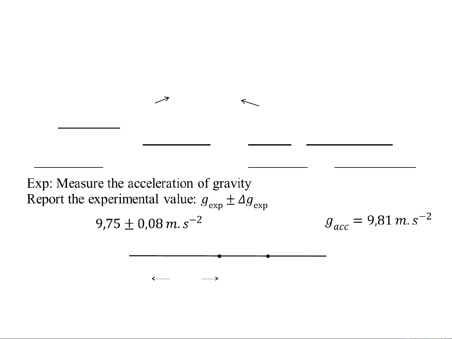
1. UNCERTAINTY vs. DISCREPANCY
When you report the result of a measurement of a quantity x, you should
also give the uncertainty x: 5.0 m ± 0.1 m x x
• The uncertainty tells you how precise you think your measurement is.
→ useful to compare your result with a "true" or accepted value
• Discrepancy is the difference between your result and accepted value Result: accepted value : g g  exp acc ] 75 81 9. 9. g  exp
The uncertainty g
in the measurement accounts exp 5
nicely for the discrepancy between g and g exp acc
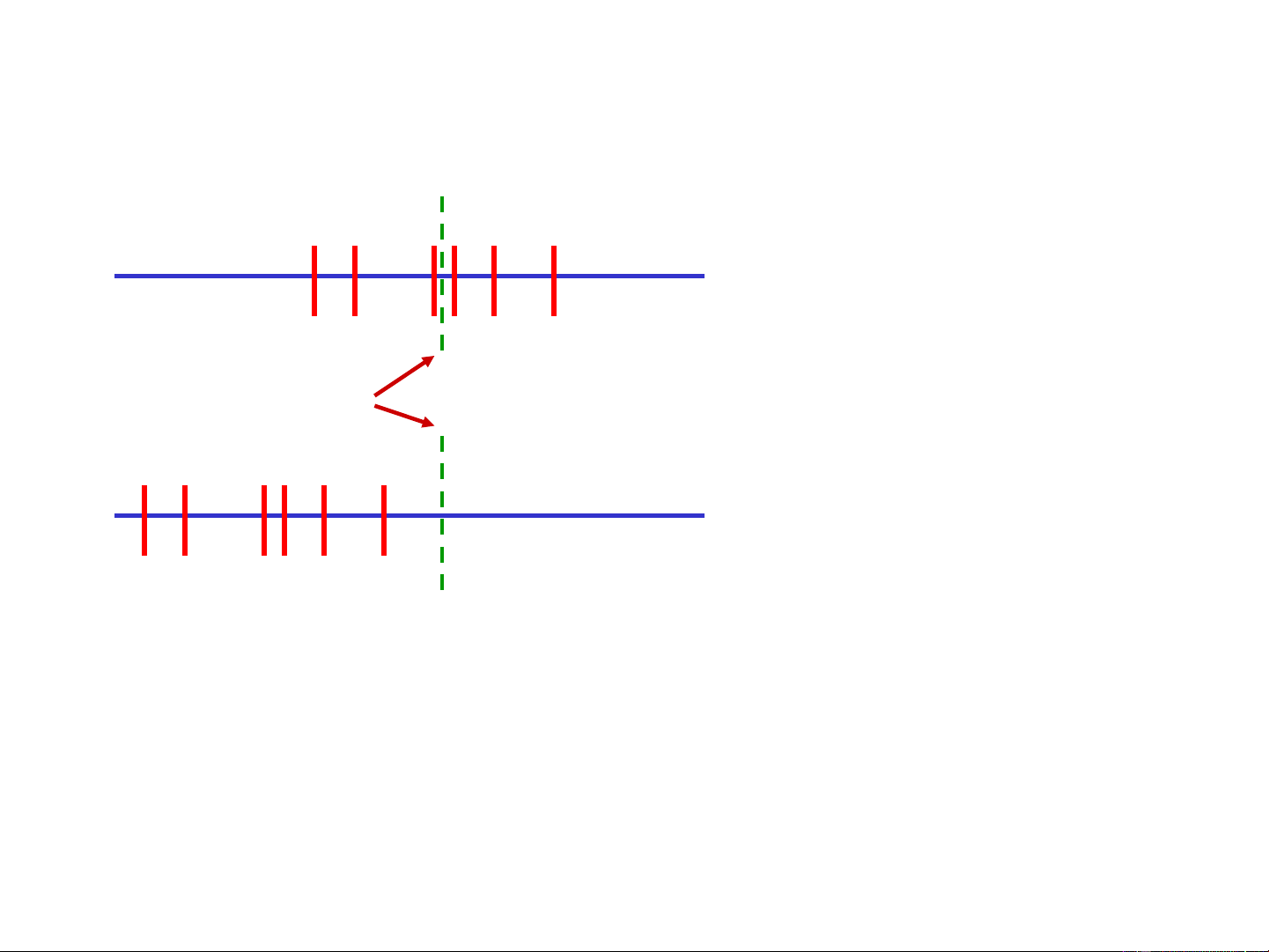
2. ORIGINS OF UNCERTAINTIES
Discrepancies between experimental values and "true" values
I. Systematic Errors are inaccuracies due to identifiable causes and
can, at least in principle, be eliminated.
a) Theoretical - due to simplifications of the model system or
approximations in the equations describing it.
b) Instrumental - e.g., a poorly calibrated instrument.
c) Environmental - e.g., factors such as inadequately controlled temperature and pressure.
d) Observational - e.g., parallax in reading a meter scale.
II. Random Uncertainties are the result of small fluctuating disturbances
which cause about half the measurements of any quantity to be too high and half to be too low. 6
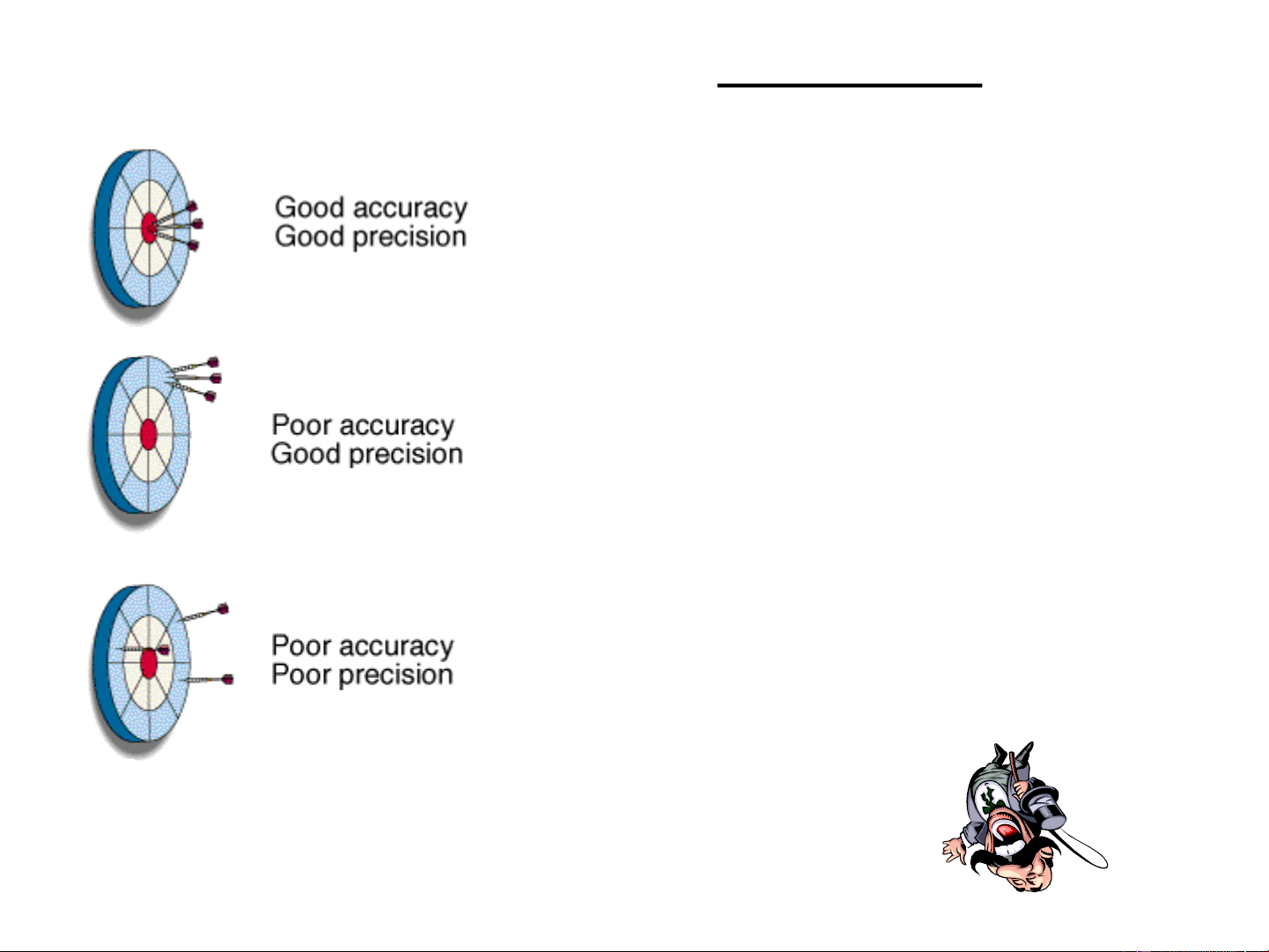
Random vs systematic errors Random errors only True value Random + systematic
• A result is said to be accurate if it is relatively free from systematic error
• A result is said to be precise if the random error is small
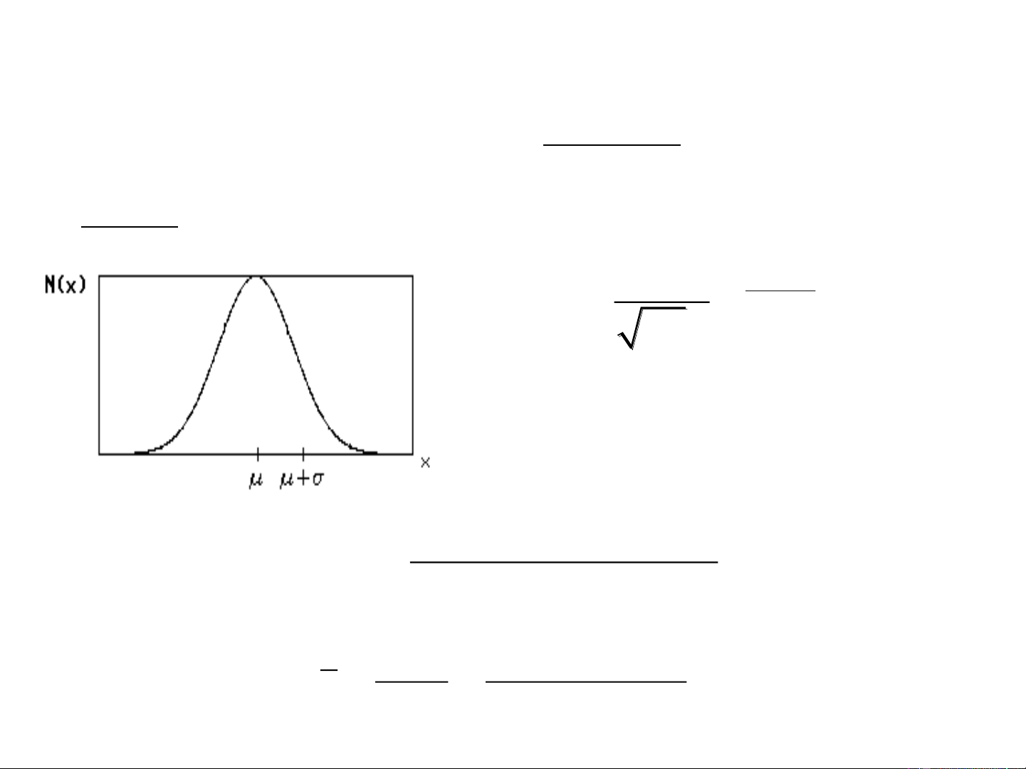
3. CHARACTERIZING A SET OF DATA: THE NORMAL DISTRIBUTION
- Make "many" measurements of a quantity x and plot the frequency
of occurrence N(x), → obtain a curve that approximates a Gaussian, or normal distribution, 2 ( x −) N0 - 2 N(x) = e 2 2
µ and  determine the position and width of the peak.
For a set of data points x , the mean of all values obtained for x i n xi x + x + +  x x i=1 1 2 n = = n n 8
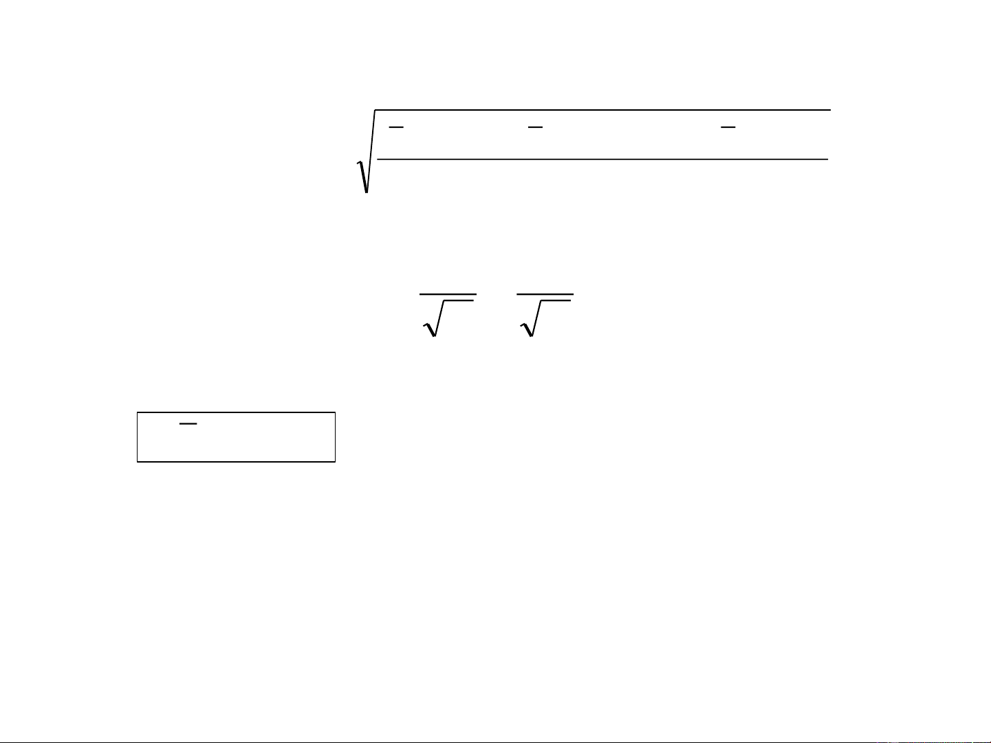
Standard deviation of a ‘single’ measurement
(x − x )2 + − + + − 1
(x x2)2 ... (x xN )2 s d . . = x = N
Standard deviation of Means: S. D. s d . . x S. . D  = N N Report of the measurements x  . D . S
S.D. in one or two significant figure 9
Propagation of Uncertainties Given: AA, BB and f = f(A,B) In general 2 2  f   f  f =  A +  B  A   B 
Addition/ subtraction: f = A + B f  = ( A  )2 + ( B  )2  
Multiplication/ division/ powers f = A B 2 2  A   B  f = f   +    A   B  10
Least Squares Fit (Linear Regression)
Measurements: (x , y ), (x , y ),………, (x , y ), N pairs of data. 1 1 2 2 N N In theory:
y = mx + b; m = slope, b = y-intercept Result of Least Squares Fit:
N x y −  x  y m i i i i = 2 N x2 −  i ( xi)
y x2 − x x y b i i i i i = 2 N x2 −  i ( xi) N
y −(mx + b) − i i 2 1 1 1 2 = 1 − r 2 i 1 r m = = m  m  N(N − ) 1 N N x r = correlati n o coefficie t n (x − x  2 2 i )2 x
b = m  + x ,  = , x i = x x 11 N N Significant figures 12
Accuracy and Precision in Measurements
Accuracy: how close a measurement is to the accepted value.
Precision: how close a series of
measurements are to one another or
how far out a measurement is taken.
A measurement can have high precision, but
not be as accurate as a less precise one. 13 Accuracy and Precision 14
Significant Figures are used to indicate the precision of a
measured number or to express the precision of a calculation with measured numbers. In any measurement the digit farthest to the right is considered to be estimated. 0 1 2 2.0 1.3 15
Rules for Determining Significant Figures in a Number
1. All non-zero numbers are significant.
2. Zeros within a number are always significant.
3. Zeros that do nothing but set the decimal point are not
significant. Both 0.000098 and 0.98 contain two significant figures.
4. Zeros that aren’t needed to hold the decimal point are
significant. For example, 4.00 has three significant figures.
5. Zeros that follow a number may be significant. 16
1. The term that is related to the reproducibility
(repeatability) of a measurement is a. accuracy.
Let’s take a “Quiz” b. precision. c. qualitative. b. precision. d. quantitative. e. property.
2. The number of significant figures in the mass measured as 0.010210 g is a. 1. b. 2. e. 5. c. 3. d. 4. e. 5. 17
3. The number of significant figures in 6.0700 x 10-4… is a. 3. b. 4. c. 5. c. 5. d. 6. e. 7.
4. How many significant figures are there in the value 0.003060? a. 7 b. 6 c. 5 d. 4 d. 4 e. 3 18
Calculations with sig. Figs.
Addition and subtraction: Look at places! 3.63 cm 13.129 cm +123.1 cm 139.859 cm = 139.9 cm significant to the 0.1 place 19
Measurement Calculations with scientific notation.
Addition/subtraction: must be placed into the same notation.
(2.3 x 103) + (3.2 x 104) = 0.23 x 104 +3.2 x 104 3.43 x 104 = 3.4 x 104 20