STATISTICAL ANALYSIS STAT3013.O11.CTTT | Tiểu luận Xác Suất Thống Kê

Vietnam National University - University of Information Technology Faculty of Information Systems
STATISTICAL ANALYSIS – STAT3013.O11.CTTT REPORT LAB 4
Lecturer: Assoc. Prof. Dr Nguyễn Đình Thuân
Teacher Assistant: Nguyễn Minh Nhựt
Student: Lê Nguyễn Gia Hưng – 21520890
Student: Nguyễn Thanh Quỳnh Tiên – 21521531
Student: Nguyễn Thiện Bảo Châu - 21521886
Vietnam National University - University of Information Technology Faculty of Information Systems INDEX I.
Task Delegation..................................................................................................................3 I.
Task 1..................................................................................................................................4 II.
Task 2............................................................................................................................14 III.
Google drive..................................................................................................................31
References.................................................................................................................................32 2
Vietnam National University - University of Information Technology Faculty of Information Systems I. Task Delegation Member Lê Nguyễn Nguyễn Nguyễn Work Gia Hưng Thanh Thiện Bảo Quỳnh Tiên Châu What x ACF and How x PACF Why x Task Example x 1 What x ARIMA How x Why x Example x Excel x ACF and R x PACF Task Python x 2 Excel x ARIMA R x Python x 3
Vietnam National University - University of Information Technology Faculty of Information Systems I. Task 1
Explanation (What, How and Why) and example of:
a) Autocovariance function (ACF) and PACF in time series
b) ARIMA (Autoregressive integrated moving average) What -
Autocorrelation Function (ACF):
The Autocorrelation Function describes the correlation between observations of a time
series at two points in time, separated by a specific lag k. Essentially, it quantifies how
a value in the time series is related to its previous values. The ACF is given by: n
∑ (Y −Y)(Y −Y) t t−k ρ =t=k+1 k n ∑ (Y −Y )2 t t =1 Where: -
ρ : Autocorrelation at lag k k
- Y : Value of the series at time t t
- Y : Mean of the series
- n : Number of observations -
Partial Autocorrelation Function (PACF):
The PACF measures the correlation between two points, controlling for the values at
all shorter lags. The PACF at lag k is the correlation between the series values k
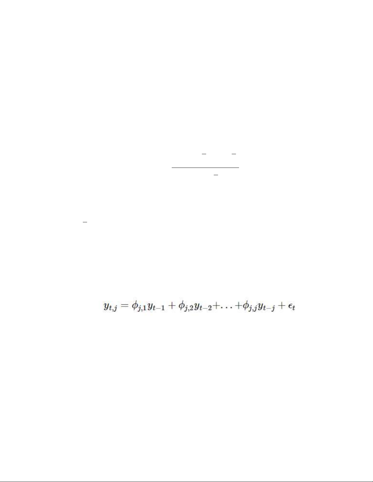
periods apart after accounting for the correlations at shorter lags 1, 2,…,k−1. Where -
y : Value of the time series at the current time (t). t , j
- ϕ , ϕ , ϕ : The PACF (Partial Autocorrelation Function) coefficients j ,1 j ,2 j , j
correspond to lags from 1 to j in the time series and is calculated by the standard
β^=(X’X)-1 X’Y coefficient.
- ϵ : the error term or residual term, represents the unexplained factors or other t
variables not considered in the model. The error term plays a role in explaining
the variability that cannot be explained by the previous time series values. How 4
Vietnam National University - University of Information Technology Faculty of Information Systems
The ACF and PACF are typically visualized using correlograms, where the x-axis
represents the lag, and the y-axis represents the correlation value. Below is a handy
way of examining a time series process to see whether an AR, MA, or ARMA
description of the process is best. Kind of plot AR(p) MA(q) ARIMA ACF behavior Falls off slowly Sharp drop after No sharp cutoff lag=q PACF behavior Sharp drop after=p Fall off slowly No sharp cutoff - ACF’s value:
ACF = -1: This indicates a perfect inverse correlation between the observations in the
time series. If one value increases, the other value decreases, and vice versa. This
implies a strong inverse correlation between the observations.
ACF = 0: This indicates no linear correlation between the observations in the time
series. The observations do not influence each other in terms of linear correlation.
ACF = 1: This indicates a strong and positive linear correlation and homogeneity
between the observations in the time series. If one value increases, the other value also
increases, and vice versa. This implies a strong linear correlation between the observations. - PACF’s value:
PACF = -1: This indicates a perfect inverse correlation between the observations in
the time series, removing indirect interactions through intermediate observations.
PACF = 0: This indicates no direct linear correlation between the observations in the
time series, removing indirect interactions through intermediate observations.
PACF = 1: This indicates a strong and direct linear correlation between the
observations in the time series, removing indirect interactions through intermediate observations.
Why do we need to use the Autocovariance Function (ACF) and Partial
Autocorrelation Function (PACF) in time series analysis?
Autocovariance Function (ACF): ACF provides insights into the temporal
dependencies present in a time series. It helps in identifying patterns such as trends, 5
Vietnam National University - University of Information Technology Faculty of Information Systems
seasonality, and cyclic behavior. ACF analysis is crucial for selecting appropriate
models like Autoregressive (AR) or Moving Average (MA) models, as it indicates the
number of past values needed to predict future values.
Partial Autocorrelation Function (PACF): PACF is particularly useful in determining
the appropriate order of the Autoregressive (AR) component in an ARIMA model. It
helps in identifying the direct influence of past values on the current value, allowing us
to build more accurate forecasting models.
ACF (Autocorrelation Function) and PACF (Partial Autocorrelation Function) comparison: ACF PACF Measures the absolute Measures the correlation
correlation between values between values in a time in a time series with series after removing Definition previous values. indirect correlations through intermediate values. Values Can range from -1 to 1. Can range from -1 to 1. ACF = -1: Perfect inverse PACF = -1: Perfect correlation. ACF = 0: No inverse correlation. PACF Interpretation linear correlation. ACF = = 0: No linear correlation. 1: Perfect linear PACF = 1: Perfect linear correlation. correlation. ACF has a slowly PACF has a cutoff pattern AR Model decreasing pattern. after a certain number of lags. ACF has a cutoff pattern PACF has a slowly MA Model after a certain number of decreasing pattern. lags. ACF helps identify the PACF helps identify the Assessment MA model. AR model. Usage Assess overall correlation. Assess direct correlation. Example:
Let suppose that we have the sales data over months:
Sales={100,120,130,110,150,140,160,170,180,190,200,210,220,230,240,250,260,270, 280,290,300,310,320,330}. 6
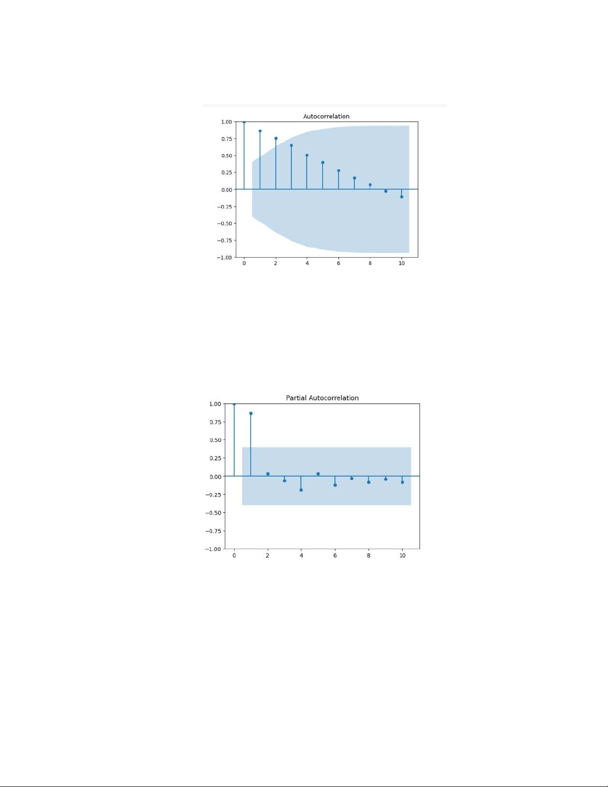
Vietnam National University - University of Information Technology Faculty of Information Systems ACF Plot:
At lag 1 and lag 2, there is a strong positive correlation. This indicates that the monthly
sales have a high correlation with the sales of the previous months.
From lag 3 onwards, the correlation values gradually decrease and approach zero. This
suggests that the correlation between the monthly sales and the sales of earlier months
weakens and becomes negligible. PACF Plot:
At lag 1 and lag 2, there is a strong positive correlation. This indicates that the monthly
sales have a strong direct correlation with the sales of the previous months, after
removing the correlation with intermediate lags.
From lag 3 onwards, the correlation values gradually decrease and approach zero. This
suggests that the direct correlation between the monthly sales and the sales of earlier
months weakens and becomes negligible. 7
Vietnam National University - University of Information Technology Faculty of Information Systems
Based on the above information, we can make some hypotheses about the
characteristics of the time series (monthly sales):
Strong historical dependence: The monthly sales depend heavily on the sales of the
previous months, especially in the short term such as lag 1 and lag 2.
Strong direct dependence: The monthly sales have a strong direct correlation with the
sales of previous months, after removing the correlation with intermediate lags.
Decreasing correlation: The correlation between the monthly sales and the sales of
earlier months decreases over time, indicating a diminishing impact of historical values on the current value b) What is ARIMA:
ARIMA stands for Autoregressive Integrated Moving Average. It is a popular time
series forecasting model that combines three components: autoregressive (AR),
differencing (I), and moving average (MA). ARIMA is designed to capture the
temporal dependencies, trends, and seasonality in a time series data.
The ARIMA model requires the time series data to be stationary before applying it.
Bringing the series into a stationary form is necessary because:
- Assumption of stationarity: The ARIMA model assumes that the time series data is
stationary to determine a more accurate model and forecasting.
- Stability of forecasts: A stationary series helps in achieving more stable forecasts
compared to non-stationary series.
- Model identification: Transforming the series into a stationary form helps in
identifying a more appropriate model and applying necessary transformations such as differencing.
In an ARIMA model, the data are differenced in order to make it stationary. A
stationary process has the property that the mean, variance and autocorrelation
structure do not change over time. If the time series is not stationary, we can often
transform it to stationarity, that is, given the series Zt, we create the new series Yi=Zi−Zi-1.
Augmented Dickey Fuller test (ADF Test) is a common statistical test used to test
whether a given Time series is stationary or not: The null hypothesis of the ADF test is
that there is a unit root present in the time series variable, indicating non-stationarity.
The alternative hypothesis is that the variable is stationary 8
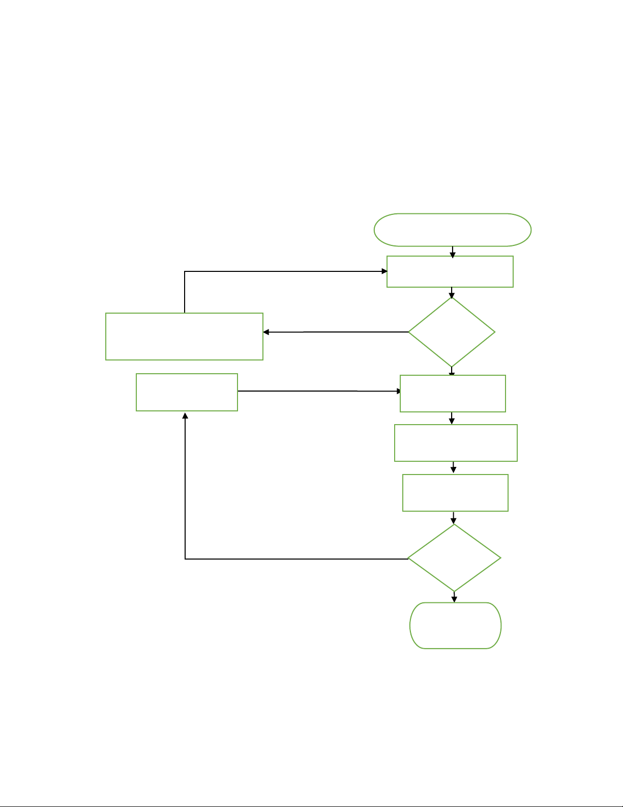
Vietnam National University - University of Information Technology Faculty of Information Systems How does ARIMA work:
We can apply Box-Jenkins method to build an ARIMA model: Time series Y=Y + Y + … + Y 1 2 n
Use of sta琀椀onary tests (ADF) No Is the 琀椀me
Making the series sta琀椀onary using series di昀昀erencing sta琀椀onary? Yes Select appropriate lags Automated ARIMA tool
Es琀椀ma琀椀on (AIC, BIC or R2) Error/Residual Analysis No Is Valida琀椀on the best 昀椀琀琀ed model? Yes Forecas琀椀ng
ARIMA model is generally denoted as ARIMA (p, d, q) and parameter p, d, q are defined as follow:
p: the lag order or the number of time lag of autoregressive model AR(p) 9
Vietnam National University - University of Information Technology Faculty of Information Systems
d: degree of differencing or the number of times the data have had subtracted with past value.
q: the order of moving average model MA(q) -
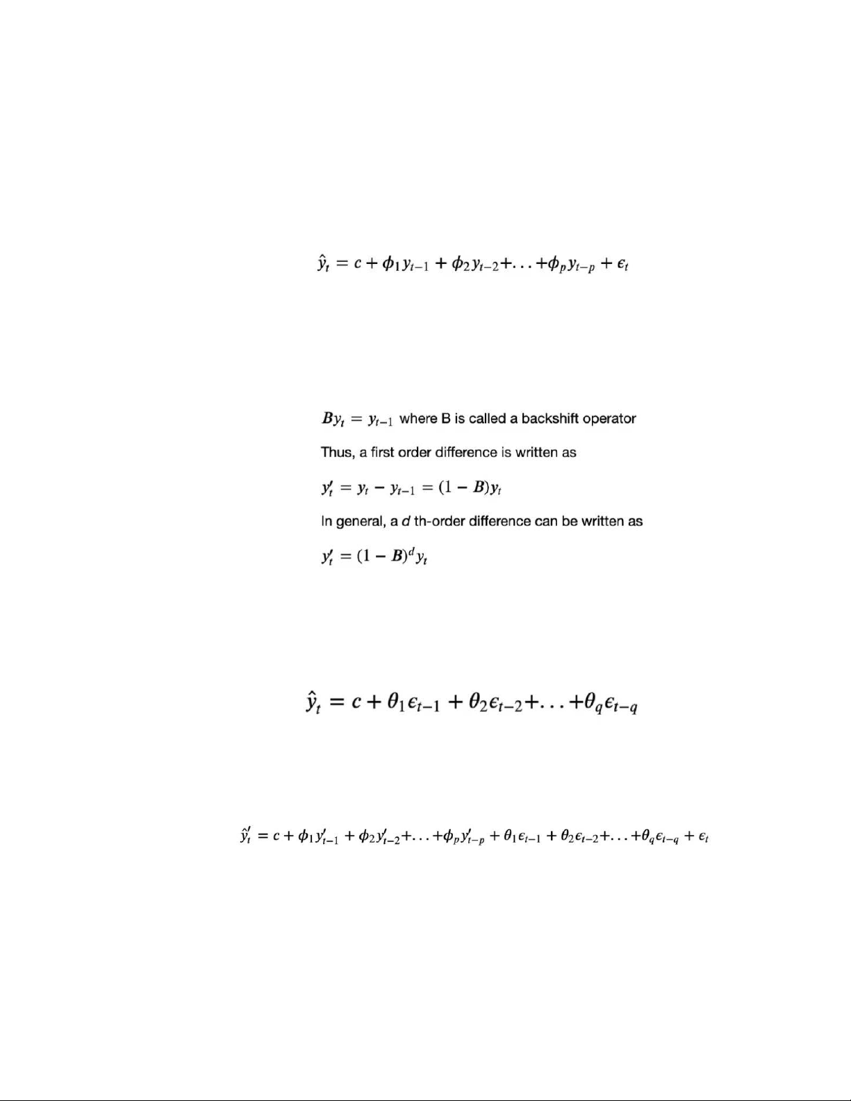
AutoRegressive - AR(p) is a regression model with lagged values of y, until p-th
time in the past, as predictors. Here, p = the number of lagged observations in the
model, ε is white noise at time t, c is a constant and φs are parameters.
- Integrated I(d) - The difference is taken d times until the original series
becomes stationary. A stationary time series is one whose properties do not
depend on the time at which the series is observed.
- Moving average MA(q) - A moving average model uses a regression-like model
on past forecast errors. Here, ε is white noise at time t, c is a constant, and θs are parameters
Combining all of the three types of models above gives the resulting ARIMA (p,d,q) model. Why is ARIMA important:
ARIMA is widely used in time series analysis and forecasting because of its flexibility
in capturing various temporal patterns and its ability to handle non-stationary data.
ARIMA models can be used to make short-term or long-term predictions and can be 10
Vietnam National University - University of Information Technology Faculty of Information Systems
applied to a wide range of domains, such as finance, economics, and weather forecasting.
This model can help individuals in forecasting for the short term. For example, one can
use it to predict a stock’s short-term price movements. Moreover, one can project a
business’s sales and interpret the seasonal changes in revenue.
It helps estimate the effect of new product launches, marketing events, and more.
This model only requires historical data.
It utilizes lagged MA for smoothing time series data.
A stationary process has the property that the mean, variance and autocorrelation
structure do not change over time.
The ARIMA (Autoregressive Integrated Moving Average) model is used for
forecasting and modeling time series data. It combines three main components:
Autoregressive (AR), Moving Average (MA), and Integrated (I). The ARIMA model is
capable of modeling and forecasting time series with correlated dependencies and
trends in the data. It is used in various fields including finance, economics, medicine,
and many other domains, to capture patterns and trends in time series data and forecast future values. Example:
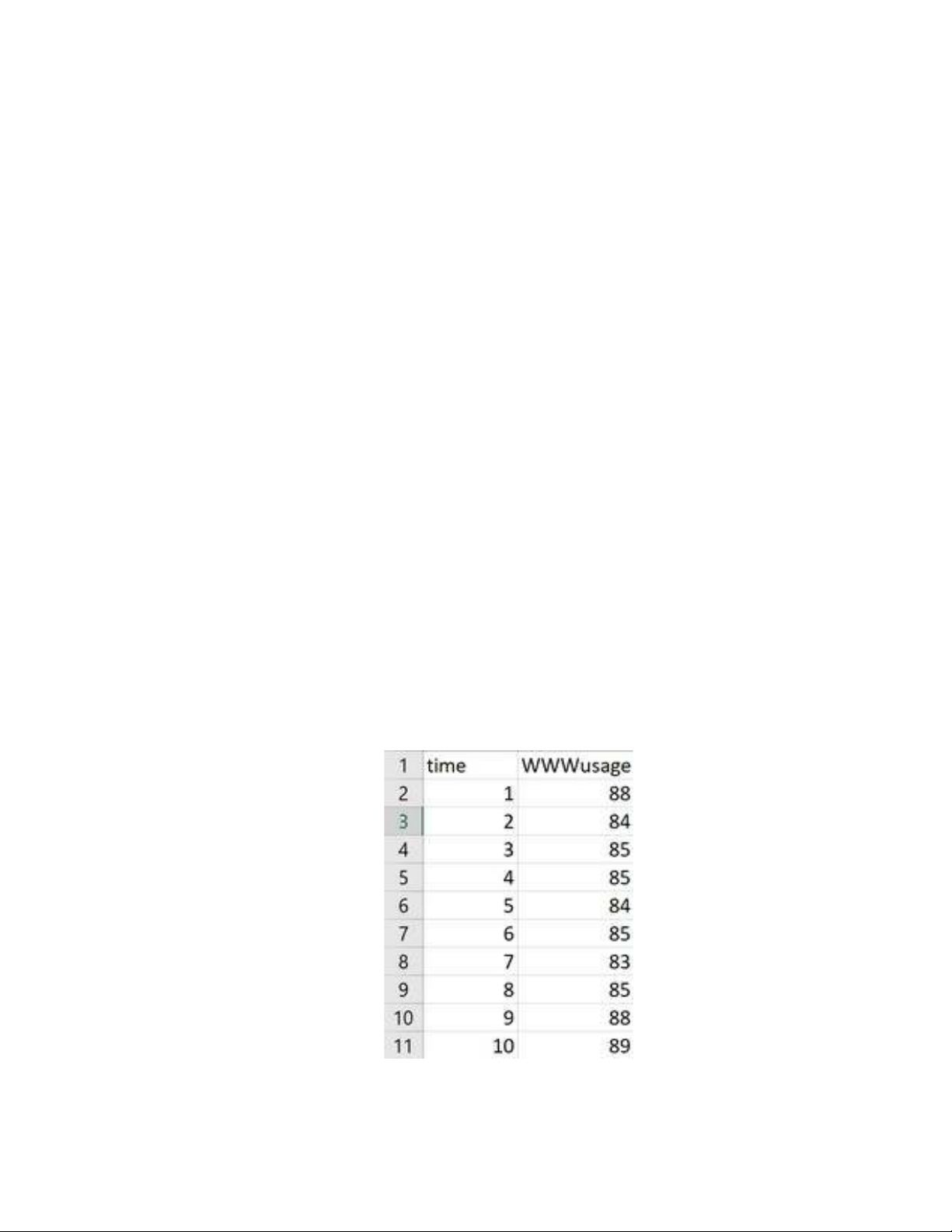
This data 100 minutes' worth of information, with each row representing the number of
users connected to the server in that minute. 11
Vietnam National University - University of Information Technology Faculty of Information Systems
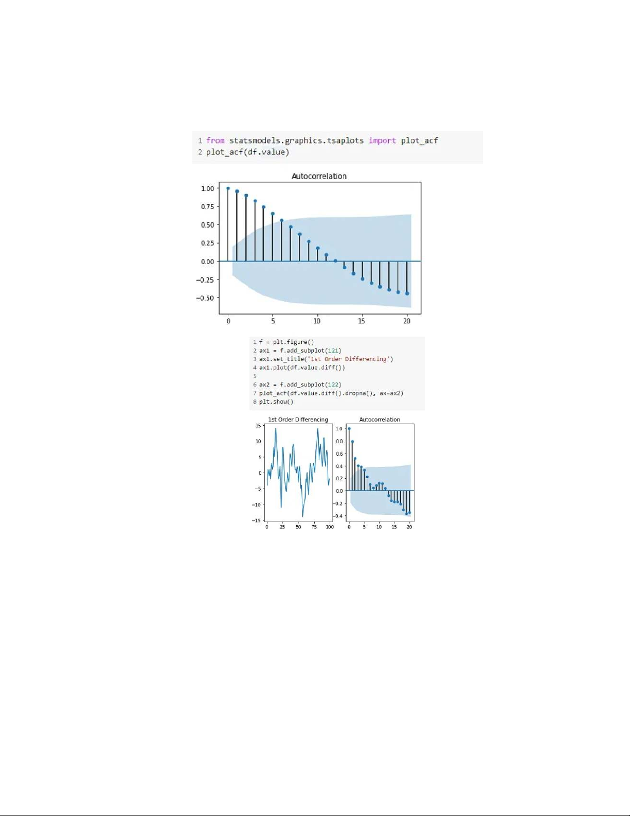
The first step would be to take care of the assumptions discussed above. For that, we
need to determine the order of differencing “d.” Let’s first check the autocorrelation
plot. The statsmodel package can help us with this
As seen above, first-order differencing shakes up autocorrelation considerably. We can
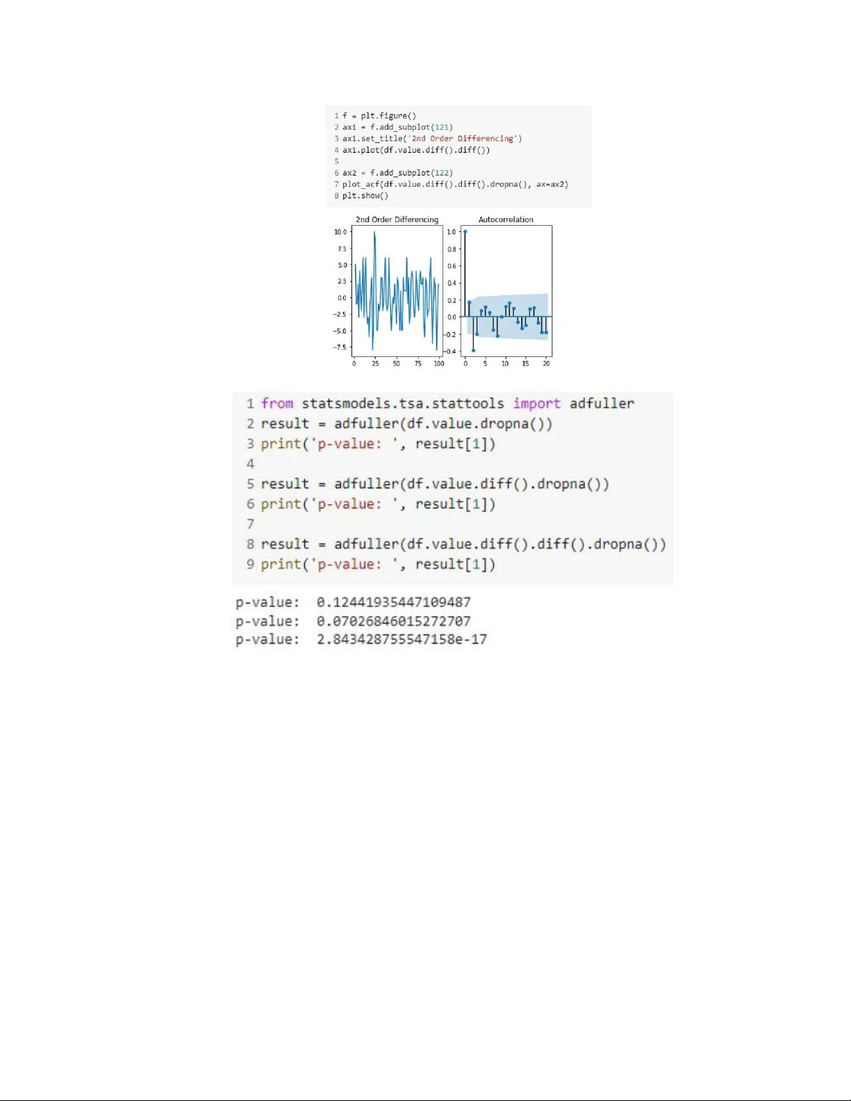
also try 2nd order differencing to enhance the stationary nature. 12
Vietnam National University - University of Information Technology Faculty of Information Systems
As we see above, after the 2nd order differencing, the p-value drops beyond the
acceptable threshold. Thus, we can consider the order of differencing (“d”) as 2. This
corresponds well with the autocorrelation line graph seen above. However, the p-value
for the 1st order is much closer to the threshold, so to be conservative, we will consider
“d” as 1 and see how the model performs.
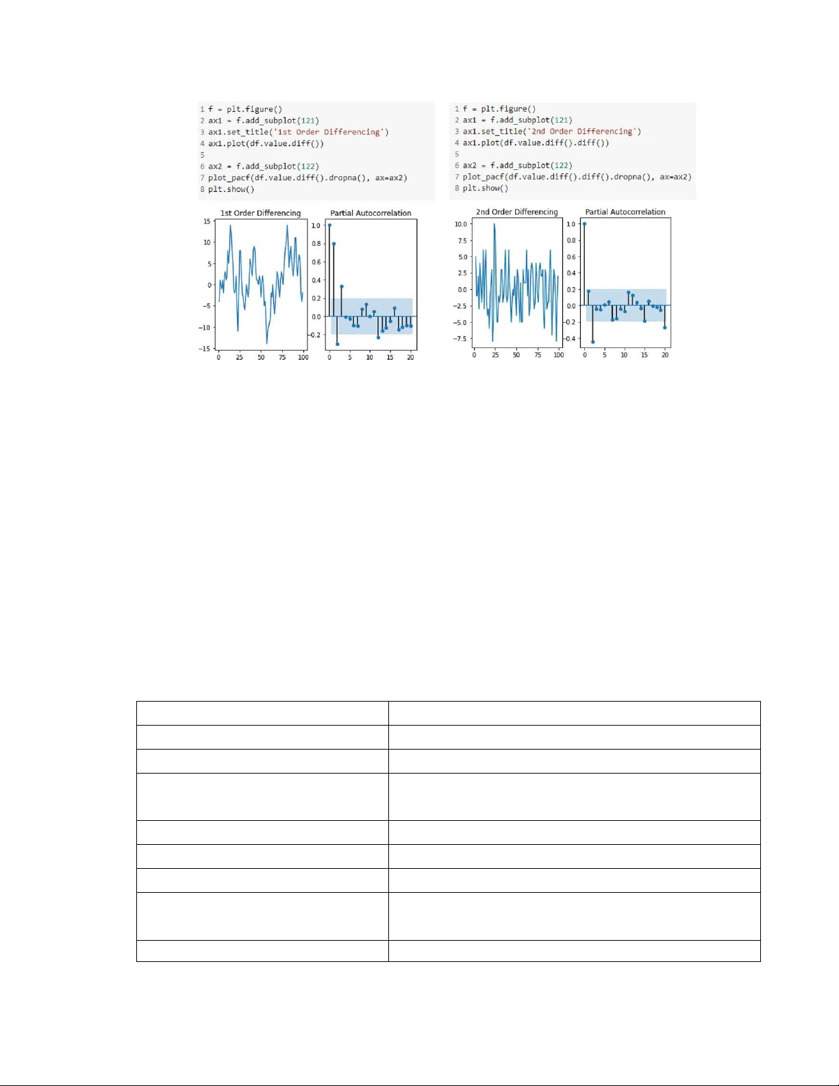
The next step in the ARIMA model is computing “p,” or the order for the
autoregressive model. We can inspect the partial autocorrelation plot, which measures
the correlation between the time-series data and a certain lag. Based on the presence or
absence of correlation, we can determine whether the lag or order is needed or not.
Thus, we determine “p” based on the most significant lag in the partial autocorrelation
plot. We can check the plot up to 2nd order difference to be sure. 13
Vietnam National University - University of Information Technology Faculty of Information Systems
In both the plots, we see the 1st lag is the most significant. Thus, we consider “p” to be 1.
Finally, “q” can be estimated similarly by looking at the ACF plot instead of the PACF
plot. Looking at the number of lags crossing the threshold, we can determine how
much of the past would be significant enough to consider for the future. The ones with
high correlation contribute more and would be enough to predict future values. From
the plots above, the moving average (MA) parameter can be set to 2.
Thus, our final Python ARIMA model can be defined as ARIMA(p=1, d=1,q= 2). II. Task 2
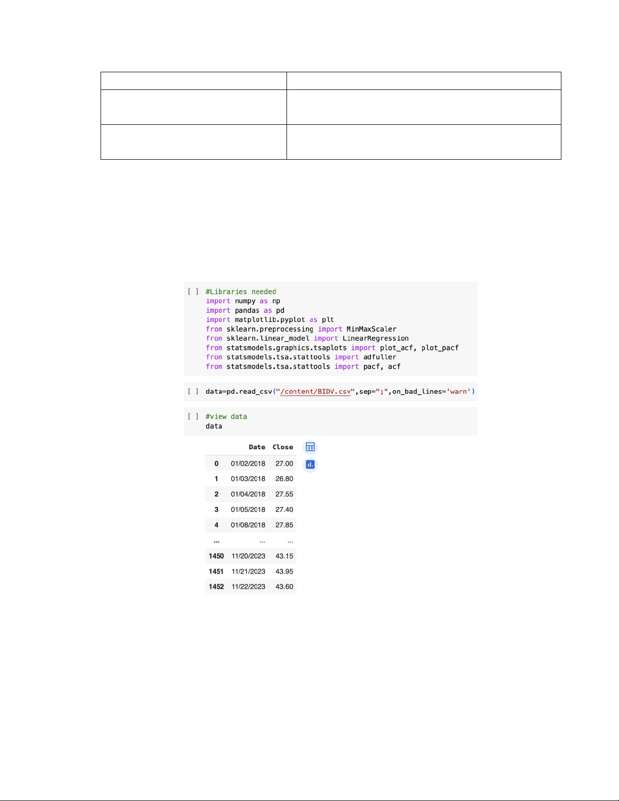
The Joint Stock Commercial Bank for Investment and Development of Vietnam
(BIDV)’s stock price is the dataset that we choose. The table below describe its attributes. Attribute Describe Date Stock trading day Close
The closing price of the stock at a certain time Change
Percentage change in the stock price from the
previous trading price to the current trading price Open
The initial price of the stock at a certain time Lowest Lowest opening price Highest Highest opening price Order-matching
Volume The total number of shares that are matched and (Shares)
traded through the order matching process Order-matching
Value The total value of the shares that are matched and 14
Vietnam National University - University of Information Technology Faculty of Information Systems (VNDmn)
traded through the order matching process Put-through Volume (Shares)
The total number of shares traded through a put- through transaction Put-through Value (VNDmn)
The total value of shares traded through a put- through transaction.
As the goal is to forecast close prices, only data relating to column “Close" will be processed.
Using MS Excel, R language and Python language to perform ACF, PACF
optional real data about/of Vietnam.
Analyzing BIDV stock price in Python
- Import libraries and data
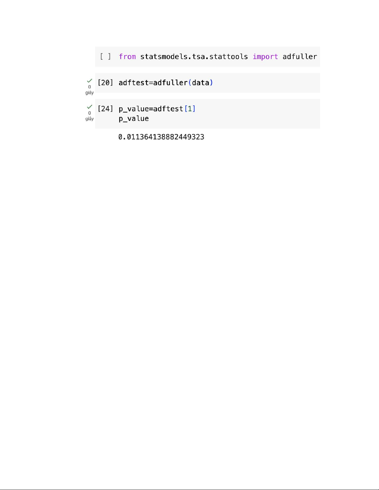
- In order to interpret the Autocorrelation Function (ACF) and Partial Autocorrelation
Function (PACF) plots effectively, it is important to ensure that the time series is
stationary. We will conduct an ADF test to check that condition. 15
Vietnam National University - University of Information Technology Faculty of Information Systems
- We use “adfuller” command to perform ADF test. The p-value is returned with 0.01
(<0.05), which means we can conclude that the time series is stationary. Therefore, we can do the ACF and PACF.
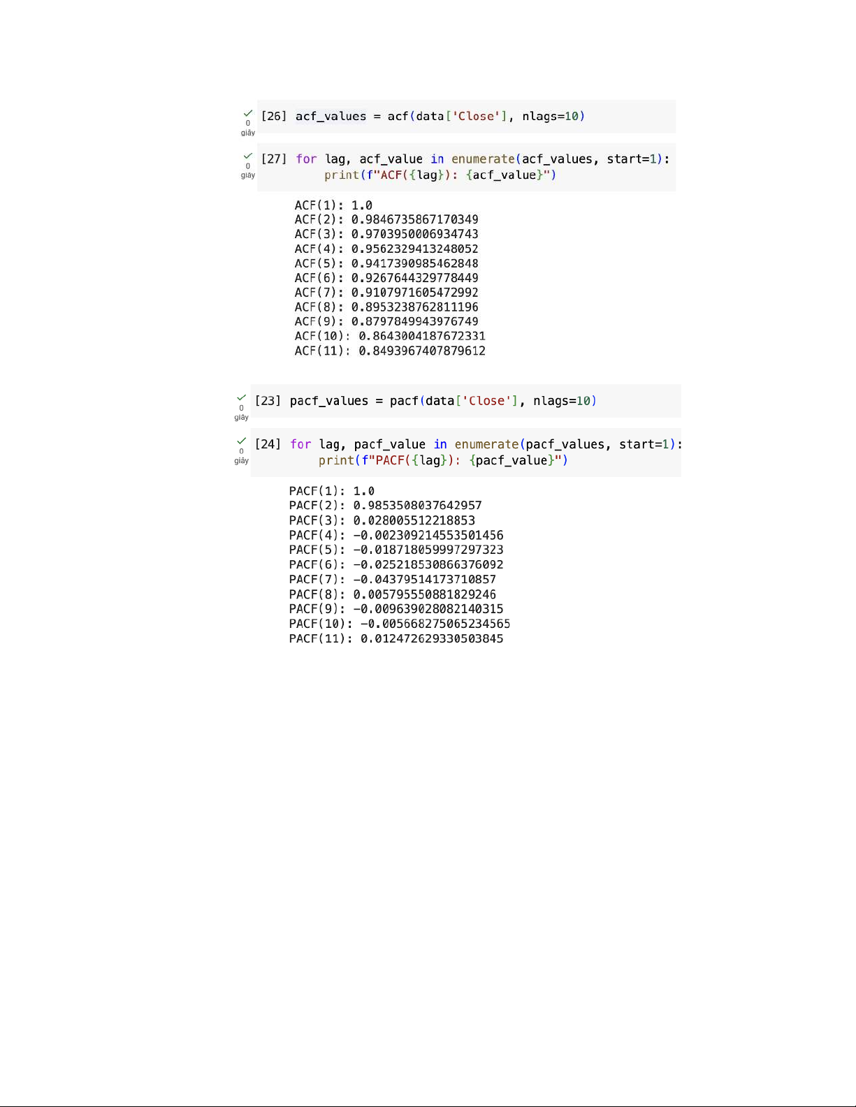
- The ACF and PACF’s values can be shown by the function: 16
Vietnam National University - University of Information Technology Faculty of Information Systems
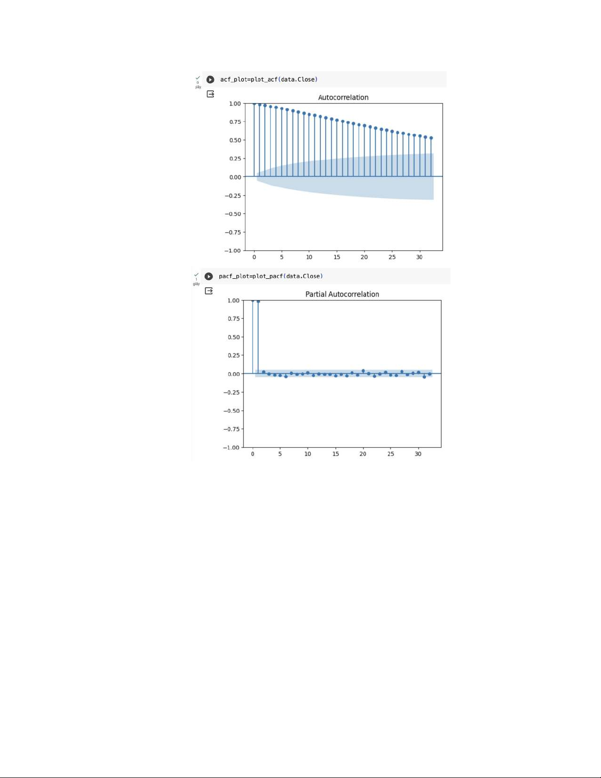
- The plot is drawn by “plot_acf” and “plot_pacf” command. 17
Vietnam National University - University of Information Technology Faculty of Information Systems
- From the plot, we can conclude:
+ The ACF plot shows a geometric decay of lags, which means the autocorrelation
values in the ACF plot decay slowly and remain significantly different from zero for
multiple lags, it suggests a correlation structure in the time series beyond random noise.
This tells us there is time series information in this dataset, and this is not just random data.
+ Looking at the PACF plot, there is only 1 signigicant lag at Lag 1.
+ According to ACF and PACF behavior, with 1 signigicant PACF lag and gradually
decaying ACF, we can conclude that the series is an AR(1) process.
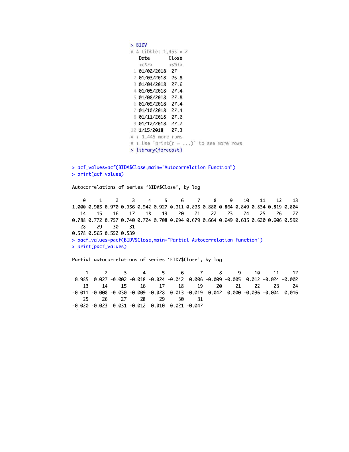
Analyzing BIDV stock price in R
- Import libraries and data 18
Vietnam National University - University of Information Technology Faculty of Information Systems
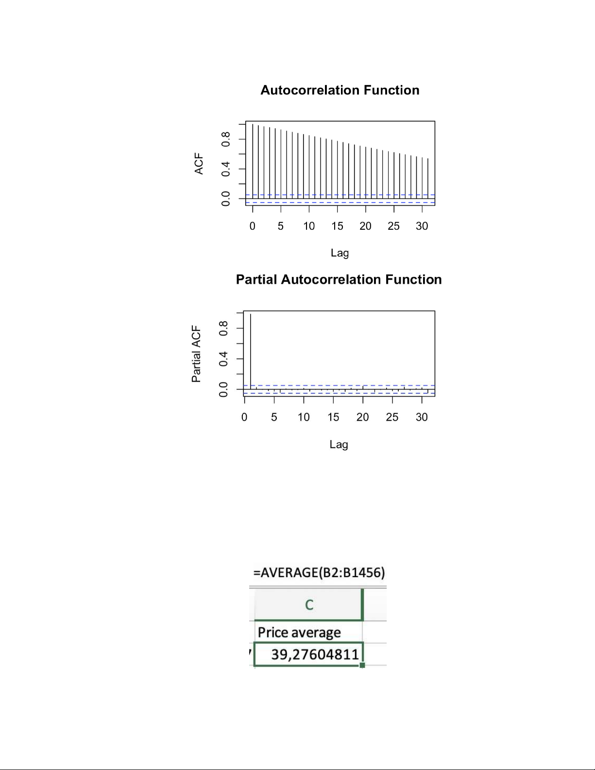
- Use “acf” and “pacf” to calculate their values and print the plots. - ACF and PACF plots: 19
Vietnam National University - University of Information Technology Faculty of Information Systems
- The result is the same as we did in Python, and we can conclude that the series is an AR(1) process.
Analyzing BIDV stock price in MS Excel ACF
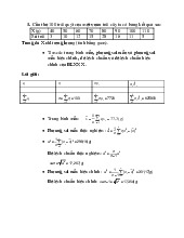
- First, we calculate the mean of data (B2:B1456 is the price’s range) 20