Statistics L2 - Descriptive Study of Bivariate Data Lecture 2 môn Xác suất thống kê| Đại học Duy Tân

14:29, 11/01/2026
Statistics L2 - Descriptive Study of Bivariate Data Lecture 2 - Studocu PROBABILITY AND STATISTICS
Lecture 2: Descriptive Study of Bivariate Data Lecturer: HồTœ Bảo
Teaching assistant: V› Thảo 14:29, 11/01/2026
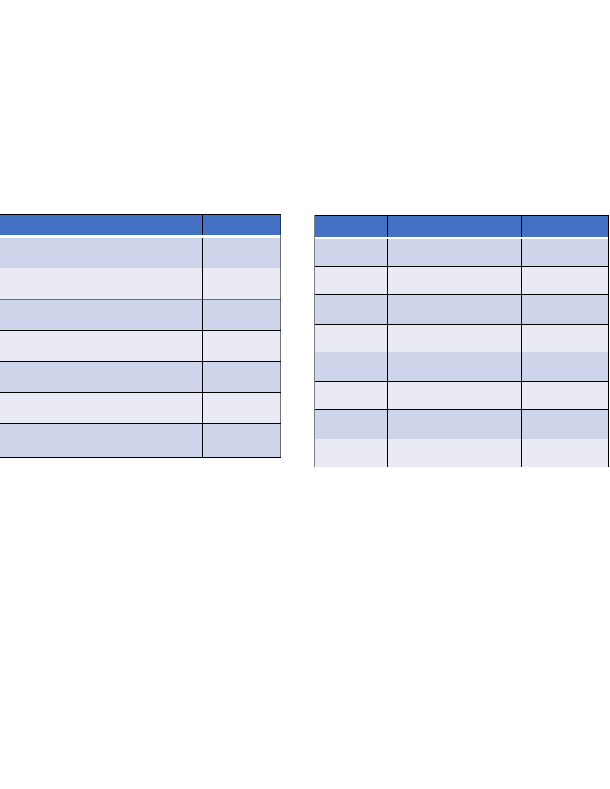
Statistics L2 - Descriptive Study of Bivariate Data Lecture 2 - Studocu What we are going to learn? Lectures Topics When Lectures Topics When Lecture 1 Digital transformation? May 9 Evaluation1 Lectures 2-7 June 1 Business Analytics? 9:20-11:45 14:50-17:10 Lecture 2 Organization and May 12 Lecture 8 Estimation June 6 Description of data 9:20-11:45 9:20-11:45 Lecture 9 Hypothesis testing June 8 Lecture 3 Bivariate relationship May 16 9:20-11:45 14:50-17:10 Lecture 10 Analysis of Categorical June 13 Lecture 4 Probability May 18 Data 9:20-11:45 14:50-17:10 Lecture 11 Comparing Two June 15 Lecture 5 Probability Distributions May 23 Treatments 14:50-17:10 9:20-11:45 Lecture 12 Analysis of Variance June 20 Lecture 6 The Normal Distribution May 25 (ANOVA) 9:20-11:45 14:50-17:10 Evaluation 2 Lectures 8-12 June 22 Lecture 7 Sampling Distribution May 30 14:50-17:10 9:20-11:45 Final June 27 examination 9:20-11:45 @Statistics, Lecture 2 3 14:29, 11/01/2026
Statistics L2 - Descriptive Study of Bivariate Data Lecture 2 - Studocu 11 rocks were collected by Apollo Astronauts and analyzed by scientists for carbon and 100 hydrogen content positive 75 association between Carbon (ppm) hydrogen 50 and carbon content 25 25 50 75 100 125 Hydrogen (ppm) @Statistics, Lecture 2 4 14:29, 11/01/2026
Statistics L2 - Descriptive Study of Bivariate Data Lecture 2 - Studocu
Descriptive study of bivariate data 1. Introduction
2. Summarization of Bivariate Categorical Data
3. Scatter Diagram of Bivariate Measurement Data 4. The Correlation Coefficient
5. Prediction of One Variable from Another @Statistics, Lecture 2 5 14:29, 11/01/2026
Statistics L2 - Descriptive Study of Bivariate Data Lecture 2 - Studocu Introduction
•Relation between smoking habit and lung cancer of adult males?
•Relation between the age of an aircraft and the time required for repair?
•By studying such bivariate or multivariate data, one typically wishes to discover if
•Any relationships exist between the variables?
•How strong the relationships appear to be?
•Whether one variable of primary interest can be effectively predicted
from information on the values of the other variables? @Statistics, Lecture 2 6 14:29, 11/01/2026
Statistics L2 - Descriptive Study of Bivariate Data Lecture 2 - Studocu
Descriptive study of bivariate data 1. Introduction
2. Summarization of Bivariate Categorical Data
3. Scatter Diagram of Bivariate Measurement Data 4. The Correlation Coefficient
5. Prediction of One Variable from Another @Statistics, Lecture 2 7 14:29, 11/01/2026
Statistics L2 - Descriptive Study of Bivariate Data Lecture 2 - Studocu
Calculation of relative frequencies
•Contingency tables (cross-tabulated data): Two traits are observed in some
qualitative categories, summarized in the form of two-way frequency table.
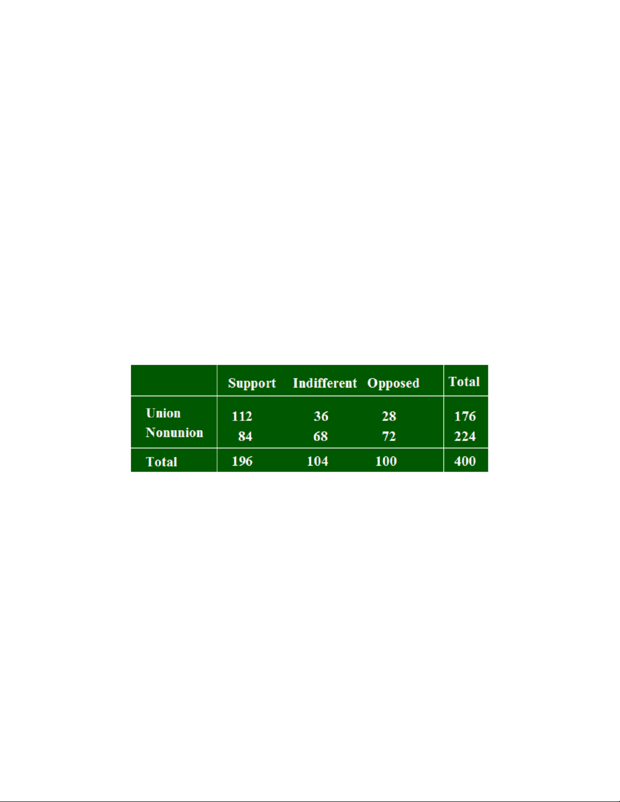
•Example: Survey by sampling 400 persons regarding union membership about
attitude toward a social welfare programs. The cross-tabulated frequency counts are presented in the table @Statistics, Lecture 2 8 14:29, 11/01/2026
Statistics L2 - Descriptive Study of Bivariate Data Lecture 2 - Studocu
Calculation of relative frequencies
Relative Frequencies (example, 112/400=.28)
Support Indifferent Opposed Total Support seems to Union .28 .09 .07 .44 be strong among Nonunion .21 .17 .18 .56 union members than non-members Total .49 .26 .25 1.00 The pertinent
Relative Frequencies by Group (example, 112/176=.636) question: Are there
Support Indifferent Opposed Total real differences of Union .636 .205 .159 1.00 attitude between Nonunion .375 .304 .321 1.00 them? @Statistics, Lecture 2 9 14:29, 11/01/2026
Statistics L2 - Descriptive Study of Bivariate Data Lecture 2 - Studocu Simpson’s paradox
•It may occur surprising and misleading conclusions when combining data from
different sources into a single table.
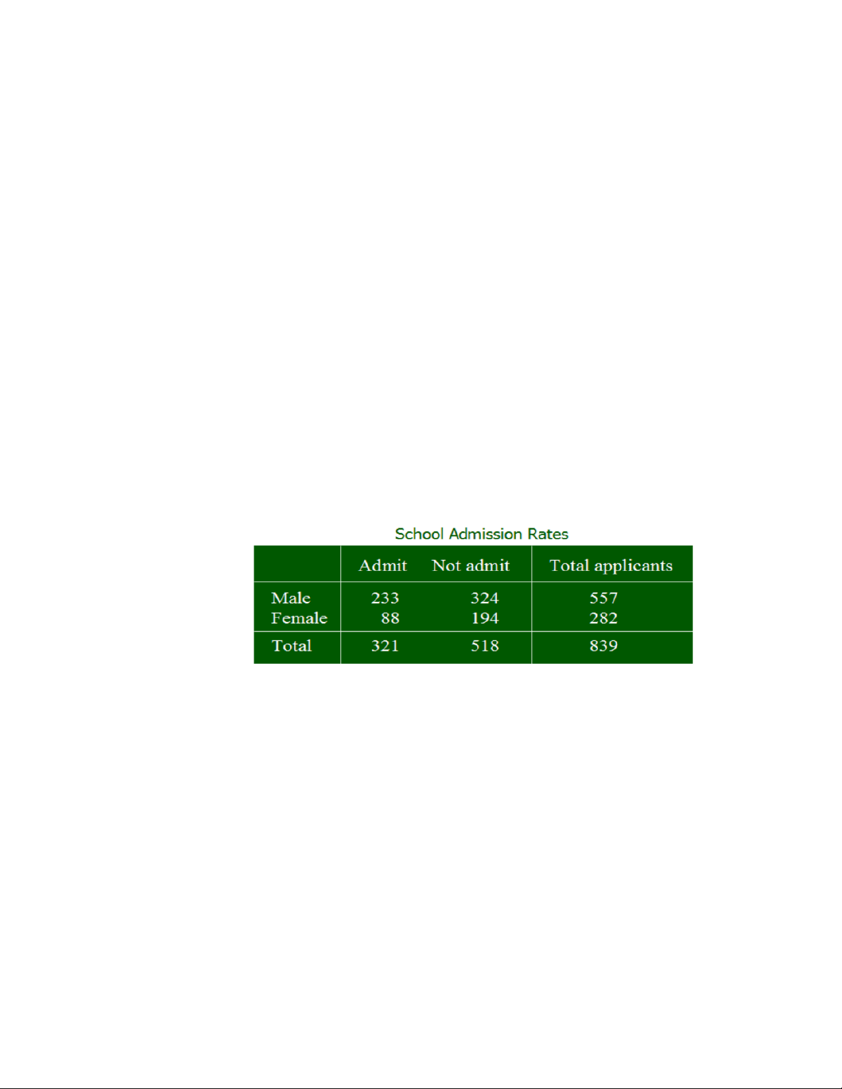
•Example: Consider graduate school admission at a large university, but use only two
departments as the whole school
•Does there appear to be a gender bias?
•Males admitted, 233/557 = .414, is greater than females admitted, 88/282= .312. Discrimination? @Statistics, Lecture 2 10 14:29, 11/01/2026
Statistics L2 - Descriptive Study of Bivariate Data Lecture 2 - Studocu Simpson’s paradox Mechanical Engineering History Not Not Admit Admit Total Admit Admit Total Male 151 35 186 Male 82 289 371 Female 16 2 18 Female 72 192 264 Total 167 37 204 Total 154 481 635
In Engineering, males admitted, 151/186 = .812, is smaller than females
admitted, 16/18 = .889. In history, 82/371 = .221 is smaller than 72/264 = .273.
females have a higher admission rates! @Statistics, Lecture 2 11 14:29, 11/01/2026
Statistics L2 - Descriptive Study of Bivariate Data Lecture 2 - Studocu Simpson’s paradox
When data from several sources are aggregated into a single table,
there is always the danger that unreported variables may cause a reversal of the findings.
http://exploringdata.cqu.edu.au/sim_par.htm @Statistics, Lecture 2 12 14:29, 11/01/2026
Statistics L2 - Descriptive Study of Bivariate Data Lecture 2 - Studocu
Descriptive study of bivariate data 1. Introduction
2. Summarization of Bivariate Categorical Data
3. Scatter Diagram of Bivariate Measurement Data 4. The Correlation Coefficient
5. Prediction of One Variable from Another @Statistics, Lecture 2 13 14:29, 11/01/2026
Statistics L2 - Descriptive Study of Bivariate Data Lecture 2 - Studocu
Scatter diagram of bivariate measurement data
•Consider a description of data sets concerning two variables, each measured on a
numerical scale, labeled xand y. For nsampling units, we have (x1, y1), (x , 2 y ) 2 , …, (x , n y ) n
•A major purpose is to answer questions as •Are the variables related?
•What form of relationship is indicated by the data?
•Can we quantify the strength of their relationship?
•Can we predict one variable from the other? @Statistics, Lecture 2 14 14:29, 11/01/2026
Statistics L2 - Descriptive Study of Bivariate Data Lecture 2 - Studocu Scatter diagram
•Scatter diagrams (scatter plot) provide a visual impression of the
nature of relation between the variables in a bivariate data
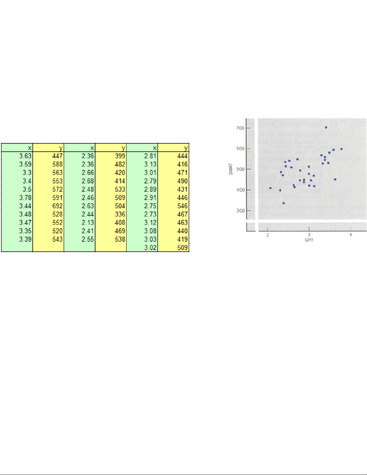
•Example: Applicants seeking admission to a Master of Business Administration program
•X = Undergraduate GPA (Grade Point Average)
•Y = Score in the Graduate Management Aptitude Test (GMAT) @Statistics, Lecture 2 15 14:29, 11/01/2026
Statistics L2 - Descriptive Study of Bivariate Data Lecture 2 - Studocu Scatter diagram
Figure shows a positive relation between x and y. That is, the
applicants with a high GPA tend to have a high GMAT @Statistics, Lecture 2 16 14:29, 11/01/2026
Statistics L2 - Descriptive Study of Bivariate Data Lecture 2 - Studocu
Descriptive study of bivariate data 1. Introduction
2. Summarization of Bivariate Categorical Data
3. Scatter Diagram of Bivariate Measurement Data 4. The Correlation Coefficient
5. Prediction of One Variable from Another @Statistics, Lecture 2 17 14:29, 11/01/2026
Statistics L2 - Descriptive Study of Bivariate Data Lecture 2 - Studocu
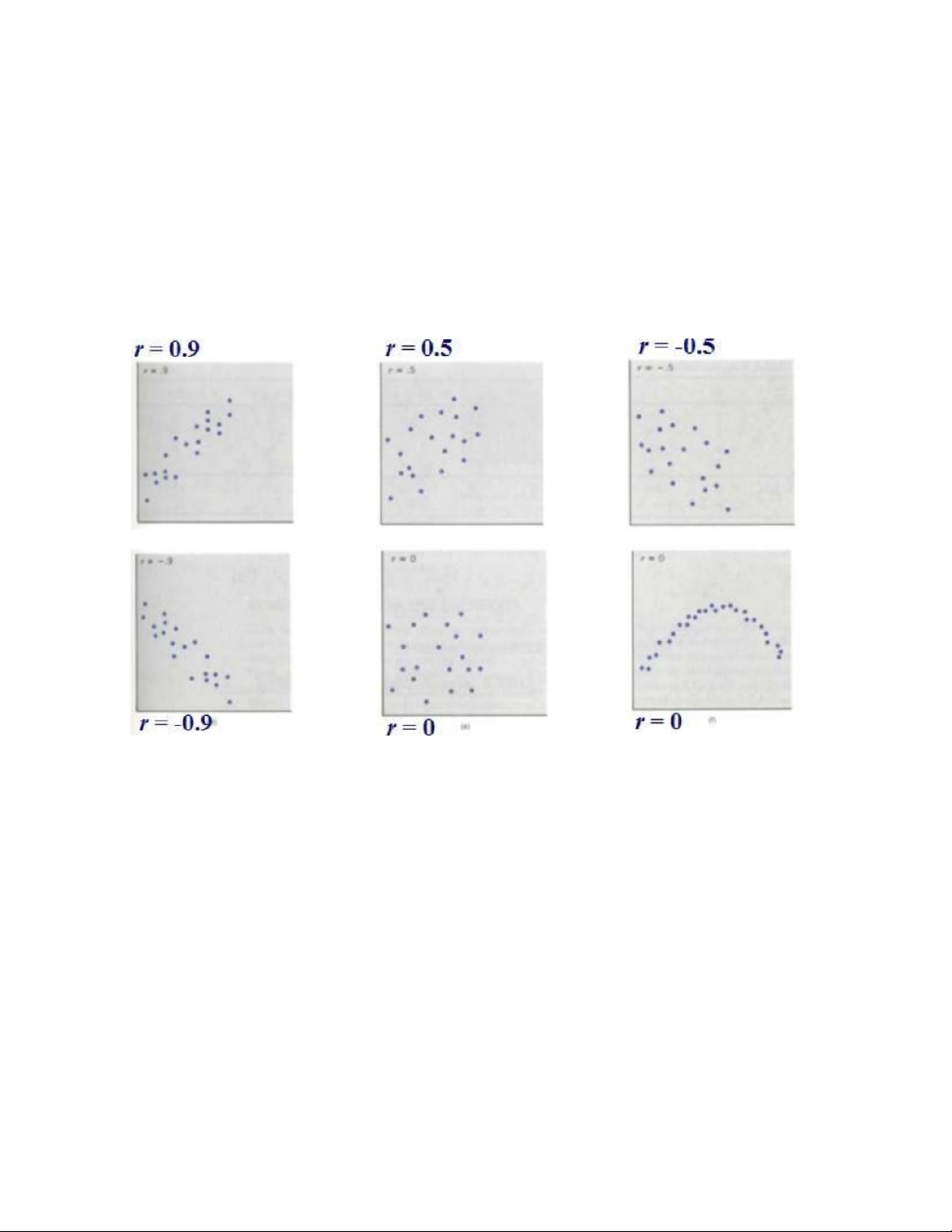
The correlation coefficient r: a measure of linear relation •-1 £r £+1
•The magnitude of rindicates the strength of a linear relation, its sign indicates the direction: •r> 0
a band of values from lower left to upper right. •r< 0
a band of values from upper left to lower right. •r= +1
all (x, y) lie on a straight line (positive slope) •r= -1
all (x, y) lie on a straight line (negative slope)
•If r close to +1 or -1, the linear relation is strong.
•If r close to zero, the linear association is very weak. @Statistics, Lecture 2 18 14:29, 11/01/2026
Statistics L2 - Descriptive Study of Bivariate Data Lecture 2 - Studocu Correlation coefficient no far from relation linear @Statistics, Lecture 2 19 14:29, 11/01/2026
Statistics L2 - Descriptive Study of Bivariate Data Lecture 2 - Studocu Correlation coefficient
•For npairs of observations (x , 1 y ) 1 , (x , 2 y2), …, (x ,
n yn) the correlation coefficient is
best interpreted in terms of standardized observations - n Observatio mean Sample x - x = i deviation standard Sample sx n = s ( ) x/( x 2) 1 n x - å=-ii 1
•Sample correlation coefficient n 1 æ- æ x x ö - ö y y r = å i ç i ÷ = n - ÷çç ç ÷÷ 1 iy1 è S S x è ø ø @Statistics, Lecture 2 20 14:29, 11/01/2026
Statistics L2 - Descriptive Study of Bivariate Data Lecture 2 - Studocu Calculation of r S r = xy Sxx Syy wher e S = xy å ( -x )x( y- y) å S = ( - x )2 x = y- xx å , S ( y)2 yy @Statistics, Lecture 2 21