













Preview text:
13 Risk, Cost of Capital, and Valuation
With more than 112,000 employees on five continents,
The WACC is the minimum return a company needs to
Germany-based BASF is a major international company. It
earn to satisfy al of its investors, including stockholders, bond-
operates in a variety of industries, including agriculture, oil
holders, and preferred stockholders. In 2010, for example,
and gas, chemicals, and plastics. In an attempt to increase
BASF pegged its cost of capital at 9 percent and earned a
value, BASF launched Vision 2020, a comprehensive plan that
company record premium of €3.9 bil ion above its cost of
included al functions within the company and chal enged and
capital. From 2011 to 2014, the company pegged its WACC
encouraged al employees to act in an entrepreneurial manner.
at 11 percent. In this chapter, we learn how to compute a
The major financial component of the strategy was that the
firm’s cost of capital and find out what it means to the firm
company expected to earn its weighted average cost of capital,
and its investors. We wil also learn when to use the firm’s cost
or WACC, plus a premium. So, what exactly is the WACC?
of capital, and, perhaps more important, when not to use it.
The goal of this chapter is to determine the rate at which cash flows of risky projects and
firms are to be discounted. Projects and firms are financed with equity, debt, and other sources
of capital, and we must estimate the cost of each of these sources in order to determine
the appropriate discount rate. We begin with the cost of equity capital. Since the analysis
here builds on beta and the capital asset pricing model (CAPM), we discuss beta in depth,
including its calculation, its intuition, and its determinants. We next discuss the cost of
debt and the cost of preferred stock. These costs serve as building blocks for the weighted
average cost of capital (R
or, more simply, WACC), which is used to discount cash WACC
flows. We calculate the WACC for a real-world company, Eastman Chemical Co. We
show how both firms and projects can be valued using WACC. Finally, we introduce flotation costs.
13.1 The Cost of Capital
Whenever a firm has extra cash, it can take one of two actions. It can pay out the cash
directly to its investors. Alternatively, the firm can invest the extra cash in a project, paying
out the future cash flows of the project. Which action would the investors prefer? If inves-
tors can reinvest the cash in a financial asset (a stock or bond) with the same risk as that 396
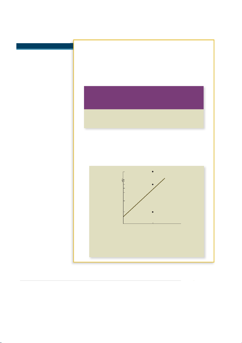
CHAPTER 13 Risk, Cost of Capital, and Valuation ■■■ 397 Figure 13.1
Corporation receives cash. Choices of a Firm It can either: Pay cash to investors with Extra Cash Inv es in t cas fi I nancial nv es h i t n cas pr as o h ject set
Investors want the firm to invest in a project only if the
expected return on the project is at least as great
as that of a financial asset of comparable risk.
of the project, the investors would desire the alternative with the higher expected return.
In other words, the project should be undertaken only if its expected return is greater than
that of a financial asset of comparable risk. This idea is illustrated in Figure 13.1. Our
discussion implies a very simple capital budgeting rule:
The discount rate of a project should be the expected return on a financial asset of comparable risk.
There are various synonyms for the discount rate. For example, the discount rate
is often called the required return on the project. This is an appropriate name, since the
project should be accepted only if the project generates a return above what is required.
Alternatively, the discount rate of the project is said to be its cost of capital. This name
is also appropriate, since the project must earn enough to pay its suppliers of capital. Our
book will use these three terms, the discount rate, the required return, and the cost of capital, synonymously.
Now imagine that all projects of the firm have the same risk. In that case, one could
say that the discount rate is equal to the cost of capital for the firm as a whole. And, if the
firm is all equity, the discount rate is also equal to the firm’s cost of equity capital.
13.2 Estimating the Cost of Equity Capital with the CAPM
We start with the cost of equity capital, which is the required return on a stockholders’
investment in the firm. The problem is that stockholders do not tell the firm what their
required returns are. So, what do we do? Luckily, the capital asset pricing model (CAPM)
can be used to estimate the required return.
Under the CAPM, the expected return on stock can be written as: R 5 R 1 b 3 (R 2 R ) (13.1) S F M F
where R is the risk-free rate and R 2 R is the difference between the expected return F M F
on the market portfolio and the riskless rate. This difference is often called the expected
excess market return or market risk premium. Note we have dropped the bar denoting
398 ■■■ PART III Risk
expectations from our expression to simplify the notation, but remember that we are
always thinking about expected returns with the CAPM.
The expected return on the stock in Equation 13.1 is based on the stock’s risk, as mea-
sured by beta. Alternatively, we could say that this expected return is the required return
on the stock, based on the stock’s risk. Similarly, this expected return can be viewed as the
firm’s cost of equity capital.
It is important to stress the symmetry between the expected return to the shareholder
and the cost of capital to the firm. Imagine a company issuing new equity to fund a capital
budgeting project. The new shareholder’s return comes in the form of dividends and capi-
tal gains. These dividends and capital gains represent costs to the firm. It is easier to see
this for dividends. Any dividend paid to a new shareholder is cash that cannot be paid to
an old shareholder. But capital gains also represent a cost to the firm. Appreciation in the
value of a firm’s stock is shared by all stockholders. If part of the capital gain goes to new
stockholders, only the remainder can be captured by the old stockholders. In other words,
the new shareholders dilute the capital gain of the old shareholders. More will be said on
this important point a little later.
While academics have long argued for the use of the CAPM in capital budgeting, how
prevalent is this approach in practice? One study1 finds that almost three-fourths of U.S.
companies use the CAPM in capital budgeting, indicating that industry has largely adopted
this approach. This fraction is likely to increase, since so many of the undergraduates
and MBAs who were taught the CAPM in school are now reaching positions of power in corporations.
We now have the tools to estimate a firm’s cost of equity capital. To do this, we need to know three things: ●
The risk-free rate, R . F ●
The market risk premium, R 2 R . M F ● The stock beta, b. EXAMPLE 13.1
Cost of Equity Suppose the stock of the Quatram Company, a publisher of col ege textbooks,
has a beta (b) of 1.3. The firm is 100 percent equity financed; that is, it has no debt. Quatram is con-
sidering a number of capital budgeting projects that wil double its size. Because these new projects
are similar to the firm’s existing ones, the average beta on the new projects is assumed to be equal
to Quatram’s existing beta. The risk-free rate is 5 percent. What is the appropriate discount rate for
these new projects, assuming a market risk premium of 8.4 percent?
We estimate the cost of equity, R , for Quatram as: S R 5 5% 1 (8.4% 3 1.3) S 5 5% 1 10.92% 5 15.92%
Two key assumptions were made in this example: (1) The beta risk of the new projects is the
same as the risk of the firm, and (2) the firm is al equity financed. Given these assumptions, it fol ows
that the cash flows of the new projects should be discounted at the 15.92 percent rate.
1John R. Graham and Campbell R. Harvey, “The Theory and Practice of Corporate Finance: Evidence from the Field,” Journal
of Financial Economics (2001), report in their Table 3 that 73.49 percent of the companies in their sample use the CAPM for capital budgeting.
CHAPTER 13 Risk, Cost of Capital, and Valuation ■■■ 399 EXAMPLE 13.2
Project Evaluation and Beta Suppose Alpha Air Freight is an al -equity firm with a beta of 1.21.
Further suppose the market risk premium is 9.5 percent, and the risk-free rate is 5 percent. We can
determine the expected return on the common stock of Alpha Air Freight from Equation 13.1. We
find that the expected return is: 5% 1 (1.21 3 9.5%) 5 16.495%
Because this is the return that shareholders can expect in the financial markets on a stock with a b of
1.21, it is the return they expect on Alpha Air Freight’s stock.
Further suppose Alpha is evaluating the fol owing non–mutual y exclusive projects: Project’s NPV Project’s Project’s When Cash Expected Internal Flows Are Project’s Cash Flows Rate of Discounted Accept or Project Beta (𝛃) Next Year Return at 16.495% Reject A 1.21 $140 40% $20.2 Accept B 1.21 120 20 3.0 Accept C 1.21 110 10 −5.6 Reject
Each project initial y costs $100. Al projects are assumed to have the same risk as the firm as a whole.
Because the cost of equity capital is 16.495 percent, projects in an al -equity firm are discounted at
this rate. Projects A and B have positive NPVs, and C has a negative NPV. Thus, only A and B wil be
accepted. This result is il ustrated in Figure 13.2.
Figure 13.2 Using the Security Market Line to Estimate the Risk-Adjusted Discount Rate for Risky Projects 40 A (NPV $20.2) 5 Accept SML region 20 B (NPV $3.0) 5 16.5 Reject region s internal rate of return (%) 10 C (NPV 5 $5.6) 2 5 Project’ 1.21 Firm’s risk (beta)
The diagonal line, cal ed the security market line, is a graphical depiction of the CAPM
and represents the relationship between the cost of equity capital and the firm’s beta. An
al -equity firm should accept a project whose internal rate of return is greater than the
cost of equity capital, and should reject a project whose internal rate of return is less than
the cost of equity capital. (This graph assumes that al projects are as risky as the firm.)
400 ■■■ PART III Risk
In the above two examples, the values for the risk-free rate, the market risk premium,
and the firm’s beta were assumed. How would we go about estimating these parameters in
practice? We will investigate each of these parameters in turn. THE RISK-FREE RATE
While no bond is completely free of the risk of default, Treasury bills and bonds in the United
States are about as close to this ideal as possible. No U.S. Treasury instrument has ever default-
ed and, at least at the present time, no instrument is considered to be in the slightest danger of
a future default. For this reason, Treasury instruments are generally considered to be risk-free.
However, as we learned from Chapter 8, there is a whole term structure of interest rates,
where the yield on any Treasury instrument is a function of that instrument’s maturity. Which
maturity should have its yield serve as the risk-free rate? The CAPM is a period-by-period
model, so a short-term rate would be a good place to start. The one-year Treasury bill rate is used
frequently.2 In a multi-period application, the expected average one-year Treasury could be used.
Another sensible approach is to select a U.S. Treasury security whose “maturity” matches
the maturity of a particular project. The match would need to be exact because while U.S.
Treasury securities are probably close to default-free, they have interest rate risk. An acceptable
rule of thumb for projects with longer term multiple cash flows is to use the yield on a U.S.
Treasury security with the average maturity of the cash flows. If you are doing international (non
U.S.) valuations, it is common practice to use a government (sovereign) bond in the “local” cur-
rency for a risk-free rate. Of course, some foreign government bonds are not actually risk-free. MARKET RISK PREMIUM
Method 1: Using Historical Data As mentioned in Chapter 10, the market
risk premium is the difference between the expected return on the market portfolio and the
risk-free rate. We can use the historical approach of Chapter 10 and settle on an estimate
of 7 percent for the market risk premium, though this number should not be interpreted as definitive.
In the current discussion, it is important to remember to use the appropriate risk-free
rate measure in defining the market risk premium. In other words, for consistency the risk-
free measure should be the same for the risk-free rate and for the market risk premium.
Method 2: Using the Dividend Discount Model (DDM) Earlier in
this chapter, we referenced a study indicating that most corporations use the CAPM for
capital budgeting. Does the CAPM imply that risk premiums must be calculated from past
returns, as we did above? The answer is no. There is another method, based on the divi-
dend discount model of an earlier chapter, for estimating the risk premium.
In Chapter 9, we pointed out that the price of a share of stock can be thought of as
equal to the present value of all of its expected future dividends. Furthermore, we noted
in that chapter that, if the firm’s dividends are expected to grow at a constant rate, , g the
price of a share of stock, P, can be written as: P 5 Div ______ R 2 g S
2How can we estimate this expected one-year rate? The anticipated average one-year rate can be estimated from the term
structure. Over the period from 1926 to 2014, the average return on 20-year Treasury bonds was 6.1 percent, and the average
return on one-year Treasury bills was 3.5 percent. Thus, the term premium, as it is called, was 6.1 2 3.5 5 2.6%. This positive
term premium is not surprising, since we know that the term structure of interest rates typically slopes upward, reflecting interest
rate risk. Suppose the yield on a 20-year Treasury bond is about 3.5 percent. This yield should reflect both the average one-year
interest rate over the next 20 years and the term premium. Thus, one can argue that the average one-year interest rate expected
over the next 20 years is 3.5 2 2.6 5 .9 percent.
CHAPTER 13 Risk, Cost of Capital, and Valuation ■■■ 401
where Div is the dividend per share expected next year, R is the discount rate or cost of S equity, and
g is the constant annual rate of expected growth in dividends. This equation can be rearranged, yielding: R 5 Div ____ 1 g S P
In words, the annual expected return on a stock is the sum of the dividend yield (5Div/P)
over the next year plus the annual expected growth rate in dividends.
Just as this formula can be used to estimate the total expected return on a stock, it can
be used to estimate the total expected return on the market as a whole. The first term on the
right-hand side is easy to estimate, since a number of print and Internet services calculate
the dividend yield for the market. For example, The Wall Street Journal recently stated that
the average dividend yield across all stocks in the Standard and Poor’s (S&P) 500 Index was
about 2.1 percent. We will use this number in our estimates.
Next, we need an estimate of the per-share growth rate in dividends across all
companies in the market. Security analysts, who are typically employees of investment
banking houses, money management firms, and independent research organizations,
study individual securities, industries, and the overall stock market. As part of their
work, they forecast dividends and earnings, as well as make stock recommendations. For
example, suppose the numbers in the Value Line (VL) Investment Survey imply a five-
year growth rate in dividends for VL’s Industrial Composite Index of about 6 percent per
year. With a dividend yield of 2.1 percent, the expected return on the market becomes
2.1% 1 6% 5 8.1%. Given a one-year yield on Treasury bills of 1.0 percent, the market
risk premium would be 8.1% 2 1.0% 5 7.1%, almost identical to the 7 percent provided by method 1.
For our firm with a beta of 1.5, the cost of capital becomes: 1.0% 1 (1.5 3 7.1%) 5 11.65%
Of course, Value Line is just one source for forecasts. More likely, a firm would either
rely on a consensus of many forecasts or use its own subjective growth estimate.
Academics have, nevertheless, long preferred the historical estimated market risk
premium for its statistical objectivity. By contrast, estimation of future dividend growth in
the DDM seems more error-prone. However, proponents of using the DDM point out that
returns in the long run can only come from the current dividend yield and future dividend
growth. Anyone who thinks that long-run stock returns will exceed the sum of these two
components is fooling himself.3 The expression, “You can’t squeeze blood out of a turnip,” applies here. 13.3 Estimation of Beta
In the previous section, we assumed that the beta of the company was known. Of course,
beta must be estimated in the real world. We pointed out earlier that the beta of a security
is the standardized covariance of a security’s return with the return on the market portfolio.
As we have seen, the formula for security i is: Cov(R , R ) σ Beta of security i 5 i M ___________ 5 i,M ____ (13.2) Var(R ) M σ 2M
3For example, see Jay Ritter, “The Biggest Mistakes We Teach,” Journal of Financial Research (Summer 2002); Eugene
Fama and Kenneth French, “The Equity Premium,” Journal of Finance (2002); and Ravi Jagannathan, E. R. McGrattan, and
A. Scherbina, “The Declining U.S. Equity Premium,” Federal Reserve Bank of Minneapolis Quarterly Review (2000).
402 ■■■ PART III Risk Measuring Company Betas
The basic method of measuring company betas is to estimate: Cov(R , R ) _____ i ___ M ___ Var( R ) M
using t 5 1, 2, . . . , T observations. Problems 1. Betas may vary over time.
2. The sample size may be inadequate.
3. Betas are influenced by changing financial leverage and business risk. Solutions
1. Problems 1 and 2 can be moderated by more sophisticated statistical techniques.
2. Problem 3 can be lessened by adjusting for changes in business and financial risk.
3. Look at average beta estimates of several comparable firms in the industry.
In words, the beta is the covariance of a security with the market, divided by the variance
of the market. Because we calculated both covariance and variance in earlier chapters,
calculating beta involves no new material. REAL-WORLD BETAS
It is instructive to see how betas are determined for actual real-world companies.
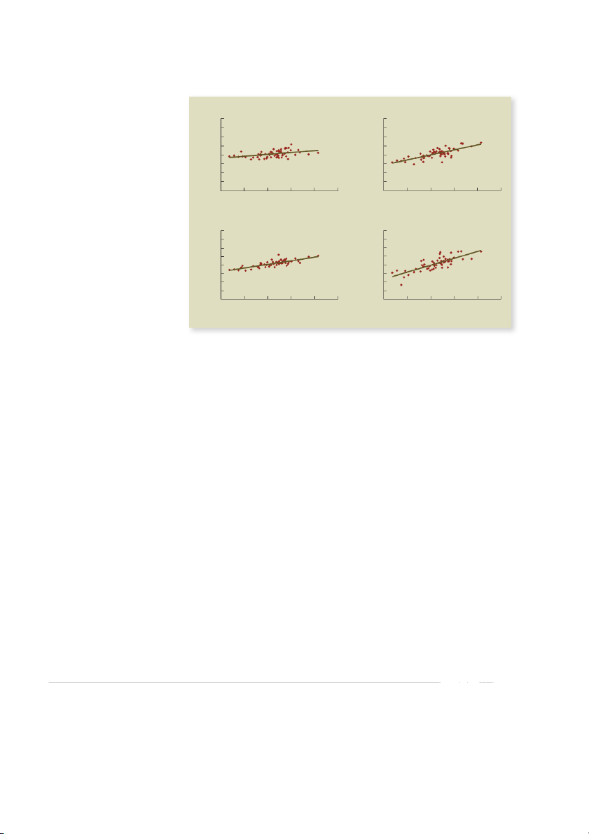
Figure 13.3 plots monthly returns for four large firms against monthly returns on the S&P
500 Index. Using a standard regression technique, we fit a straight line through the data
points. The result is called the “characteristic” line for the security. The slope of the char-
acteristic line is beta. Though we have not shown it in the table, we can also determine the
intercept (commonly called alpha) of the characteristic line by regression.
We use five years of monthly data for each plot. Although this choice is arbitrary, it
is in line with calculations performed in the real world. Practitioners know that the accu-
racy of the beta coefficient is suspect when too few observations are used. Conversely,
because firms may change their industry over time, observations from the distant past are out of date.
We stated in a previous chapter that the average beta across all stocks in an index is 1.
Of course, this need not be true for a subset of the index. For example, of the four securi-
ties in our figure, two have betas above 1 and two have betas below 1. Because beta is a
measure of the risk of a single security for someone holding a large, diversified portfolio,
our results indicate that Procter & Gamble has relatively low risk and Prudential has rela- tively high risk. STABILITY OF BETA
We have stated that the beta of a firm is likely to change if the firm changes its industry. It
is also interesting to ask the reverse question: Does the beta of a firm stay the same if its industry stays the same?
CHAPTER 13 Risk, Cost of Capital, and Valuation ■■■ 403 Figure 13.3
Proctor & Gamble versus S&P 500—Beta .41
Chevron versus S&P 500—Beta 1.15 Plots of Five Years 40% 40% of Monthly Returns 30% 30% (2010–2014) on Four ) 20% ) 20% Individual Securities 10% (% 10% against Five Years of rn 0% 0% u urn (% –10% –10% Monthly Returns on Ret Ret –20% –20% the Standard & Poor’s –30% –30% (S&P) 500 Index –40% –40% –10% –5% 0% 5% 10% 15% –10% –5% 0% 5% 10% 15% S&P 500 return (%) S&P 500 return (%)
Costco versus S&P 500—Beta .85
Prudential versus S&P 500—Beta 1.61 40% 40% 30% 30% ) 20% 20% ) 10% 10% urn (% 0% 0% urn (% –10% –10% Ret Ret –20% –20% –30% –30% –40% –40% –10% –5% 0% 5% 10% 15% –10% –5% 0% 5% 10% 15% S&P 500 return (%) S&P 500 return (%)
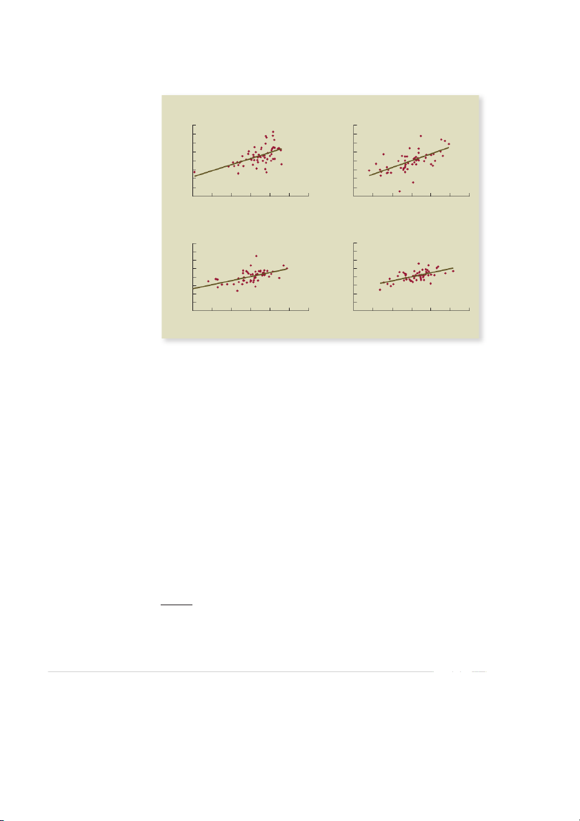
Take the case of Microsoft, which has remained in the same industry for many
decades. Figure 13.4 plots the returns on Microsoft and the returns on the S&P 500
for four five-year periods. As can be seen from the figure, Microsoft’s beta varies
from period to period. However, this movement in beta is probably nothing more than
random variation. Thus, for practical purposes, Microsoft’s beta has been approximately
constant over the two decades covered in the figure. Although Microsoft is just one
company, most analysts argue that betas are generally stable for firms remaining in the same industry.
However, this is not to say that, as long as a firm stays in the same industry, its beta
will never change. Changes in product line, changes in technology, or changes in the mar-
ket may affect a firm’s beta. Furthermore, as we will show in a later section, an increase
in the leverage of a firm (i.e., the amount of debt in its capital structure) will increase the firm’s beta. USING AN INDUSTRY BETA
Our approach to estimating the beta of a company from its own past data may seem com-
monsensical to you. However, it is frequently argued that people can better estimate a firm’s
beta by involving the whole industry. Consider Table 13.1, which shows the betas of some
prominent firms in the software industry. The average beta across all of the firms in the table
is 1.08. Imagine a financial executive at Computer Sciences trying to estimate the firm’s beta.
Because beta estimation is subject to large, random variation in this volatile industry, the
404 ■■■ PART III Risk Figure 13.4 1991–1995 2000–2004 Plots of Monthly
Microsoft versus S&P 500—Beta 1.37
Microsoft versus S&P 500—Beta 1.53 Returns on Microsoft 40% 40% Corporation against 30% 30% Returns on the ) 20% ) 20% Standard & Poor’s 10% (% 10% rn 0% 0% 500 Index for etu –10% eturn (% –10% Four Consecutive R R –20% –20% Five-Year Periods –30% –30% –40% –40% –15% –10% –5% 0% 5% 10% 15% –15% –10% –5% 0% 5% 10% 15% S&P 500 return (%) S&P 500 return (%) 2005–2009 2010–2014
Microsoft versus S&P 500—Beta .96
Microsoft versus S&P 500—Beta .95 40% 40% 30% 30% ) 20% ) 20% 10% 10% 0% 0% eturn (% –10% eturn (% –10% R R –20% –20% –30% –30% –40% –40% –15% –10% –5% 0% 5% 10% 15% –15% –10% –5% 0% 5% 10% 15% S&P 500 return (%) S&P 500 return (%)
executive may be uncomfortable with the estimate of 1.30. However, the error in beta esti-
mation on a single stock is much higher than the error for a portfolio of securities. Thus, the
executive of Computer Sciences may prefer the average industry beta of 1.08 as the estimate
of his or her own firm’s beta.4
Assuming a risk-free rate of 1.0 percent and a risk premium of 7 percent, Computer
Sciences might estimate its cost of equity capital as: 1.0% 1 1.30 3 7% 5 10.1%
However, if Computer Sciences believed the industry beta contained less estimation error,
it could estimate its cost of equity capital as: 1.0% 1 1.08 3 7% 5 8.56%
The difference is substantial here, presenting a difficult choice for a financial executive at Computer Sciences.
While there is no formula for selecting the right beta, there is a very simple guideline.
If you believe that the operations of a firm are similar to the operations of the rest of the
4Actually, one should adjust for leverage before averaging betas, though not much is gained unless leverage ratios differ signifi-
cantly. Adjustment for leverage will be discussed in later chapters.
CHAPTER 13 Risk, Cost of Capital, and Valuation ■■■ 405 Table 13.1 Company Beta
Betas for Firms in the Computer Software Microsoft .98 Industry Apple, Inc. .94 Automatic Data Processing .86 Oracle Corp. 1.41 Computer Sciences 1.30 CA, Inc. 1.34 Fiserv, Inc. 1.03 Accenture, Ltd. 1.18 Symantec Corp. .91 Paychex, Inc. .89 Equal y weighted portfolio 1.08
SOURCE: www.reuters.com December 16, 2014.
industry, you should use the industry beta simply to reduce estimation error. However, if
an executive believes that the operations of the firm are fundamentally different from those
in the rest of the industry, the firm’s beta should be used.
13.4 Determinants of Beta
The regression analysis approach in Section 13.3 doesn’t tell us where beta comes from.
Of course, the beta of a stock does not come out of thin air. Rather, it is determined by
the characteristics of the firm. We consider three factors: The cyclical nature of revenues,
operating leverage, and financial leverage. CYCLICALITY OF REVENUES
The revenues of some firms are quite cyclical. That is, these firms do well in the
expansion phase of the business cycle and do poorly in the contraction phase.
Empirical evidence suggests high-tech firms, retailers, and automotive firms fluctu-
ate with the business cycle. Firms in industries such as utilities, railroads, food, and
airlines are less dependent on the cycle. Because beta measures the responsiveness of
a stock’s return to the market’s return, it is not surprising that highly cyclical stocks have high betas.
It is worthwhile to point out that cyclicality is not the same as variability. For example,
a moviemaking firm has highly variable revenues because hits and flops are not easily pre-
dicted. However, because the revenues of a studio are more dependent on the quality of its
releases than the phase of the business cycle, motion picture companies are not particularly
cyclical. In other words, stocks with high standard deviations need not have high betas, a point we have stressed before.
406 ■■■ PART III Risk OPERATING LEVERAGE
We distinguished fixed costs from variable costs in Chapter 7. We mentioned that fixed
costs do not change as quantity changes. Conversely, variable costs increase as the quan-
tity of output rises. Firms often face a trade-off between fixed and variable costs. For
example, a firm can build its own factory, incurring a high level of fixed costs in the pro-
cess. Alternatively, the firm can outsource production to a supplier, typically generating
lower fixed costs but higher variable costs. Fixed costs tend to magnify the impact of sales
cyclicality. Fixed costs must be paid, even at a low level of sales, leaving the firm with the
possibility of large losses. And with fixed costs replacing variable costs, any additional
sales generate low marginal costs, leaving the firm with a substantial increase in profit.
Firms with high fixed costs and low variable costs are generally said to have high
operating leverage. Conversely, firms with low fixed and high variable costs have low
operating leverage. Operating leverage magnifies the effect of the cyclicality of a firm’s
revenues on beta. That is, a firm with a given sales cyclicality will increase its beta if fixed
costs replace variable costs in its production process. FINANCIAL LEVERAGE AND BETA
As suggested by their names, operating leverage and financial leverage are analogous con-
cepts. Operating leverage refers to the firm’s fixed costs of production. Financial leverage
is the extent to which a firm relies on debt, and a levered firm is a firm with some debt in
its capital structure. Because a levered firm must make interest payments regardless of the
firm’s sales, financial leverage refers to the firm’s fixed costs of finance.
Just as an increase in operating leverage increases beta, an increase in financial lever-
age (i.e., an increase in debt) increases beta. To see this point, consider a firm with some
debt and some equity in its capital structure. Further, imagine an individual who owns all
the firm’s debt and all its equity. In other words, this individual owns the entire firm. What
is the beta of her portfolio of the firm’s debt and equity?
As with any portfolio, the beta of this portfolio is a weighted average of the betas of
the individual items in the portfolio. Let B stand for the market value of the firm’s debt and
S stand for the market value of the firm’s equity. We have: β 5 β 5 S ______ 3 β 1 B ______ 3 β (13.3) Portfolio Asset B 1 S Equity B 1 S Debt where b
is the beta of the stock of the levered firm. Notice that the beta of debt, b , Equity Debt
is multiplied by By(B 1 S), the percentage of debt in the capital structure. Similarly, the
beta of equity is multiplied by the percentage of equity in the capital structure. Because
the portfolio contains both the debt of the firm and the equity of the firm, the beta of
the portfolio can be thought of as the beta of the common stock had the firm been all
equity. In practice, this beta is called the asset beta because its value is dependent only on the assets of the firm.
The beta of debt is very low in practice. If we make the common assumption that the
beta of debt is zero (or very close to zero), we have: β 5 S ______ 3 β (13.4) Asset B 1 S Equity
Because Sy(B 1 S) must be below 1 for a levered firm, it follows that b , b . Asset Equity
Rearranging this equation, we have: β 5 β ( 1 1 B __ Equity Asset S )
CHAPTER 13 Risk, Cost of Capital, and Valuation ■■■ 407
The equity beta will always be greater than the asset beta with financial leverage (assuming
the asset beta is positive).5 In other words, the equity beta of a levered firm will always be
greater than the equity beta of an otherwise identical all-equity firm.
Which beta does regression analysis estimate, the asset beta or the equity beta?
Regression, as performed in Section 13.3 and also in the real world, provides us with an
equity beta because the technique uses stock returns as inputs. We must transform this
equity beta using Equation 13.4 to arrive at the asset beta. (Of course, the two betas are
the same for an all-equity firm.) EXAMPLE 13.3
Asset versus Equity Betas Consider a tree growing company, Rapid Cedars, Inc., which is cur-
rently al equity and has a beta of .8. The firm has decided to move to a capital structure of one part
debt to two parts equity. Because the firm is staying in the same industry, its asset beta should remain
at .8. However, assuming a zero beta for its debt, its equity beta would become: β 5 β ( 1 1 B__ Equity Asset S ) 1.2 1 5 .8 ( 1 1 _ _ 2)
If the firm had one part debt to one part equity in its capital structure, its equity beta would be: 1.6 5 .8(1 1 1)
However, as long as it stays in the same industry, its asset beta would remain at .8. The effect of
leverage, then, is to increase the equity beta.
13.5 The Dividend Discount Model Approach
In Section 13.2, we showed how the CAPM could be used to determine a firm’s cost of
capital. Among other inputs, we needed an estimate of the market risk premium. One
approach used the dividend discount model (DDM) to forecast the expected return on the
market as a whole, leading to an estimate of this risk premium. We now use the DDM to
estimate the expected return on an individual stock directly.
Our discussion in Section 13.2 on the DDM led to the following formula: R 5 Div ____ 1 g S P
where P is the price per share of a stock, Div is the dividend per share to be received
next year, R is the discount rate, and
g is the expected annual growth rate in dividends S
per share. The equation tells us that the discount rate on a stock is equal to the sum of the
5It can be shown that the relationship between a firm’s asset beta and its equity beta with corporate taxes is: β 5 β
[ 1 1 (1 2 t ) B _ _ Equity Asset C S ]
In this expression, t is the corporate tax rate. Tax effects are considered in more detail in later chapters. C
408 ■■■ PART III Risk
stock’s dividend yield (5Div/P) and its expected growth rate of dividends. Thus, in order
to apply the DDM to a particular stock, we must estimate both the dividend yield and the expected growth rate.
The dividend yield is relatively easy to forecast. Security analysts routinely provide
forecasts of next year’s dividend for many stocks. Alternatively, we can set next year’s
dividend as the product of last year’s dividend and 1 1 ,
g using approaches to estimate g
that we describe below. The price per share of any publicly traded stock can generally be
determined from either financial newspapers or the Internet.
The expected growth rate of dividends can be estimated in one of three ways. First, we
can calculate the firm’s historical growth rate in dividends from past data. For some firms,
this historical growth rate may be a serviceable, though clearly imperfect, estimate of the
future growth rate. Second, in Chapter 9, we argued that the growth rate in dividends can be expressed as:
g 5 Retention ratio 3 ROE
where the retention ratio is the ratio of retained earnings to earnings, and ROE stands for
return on equity. Return on equity is the ratio of earnings to the accounting book value
of the firm’s equity. All the variables needed to estimate both the retention ratio and ROE
can be found on a firm’s income statement and balance sheet. Third, security analysts
commonly provide forecasts of future growth. However, analysts’ estimates are generally
for five-year growth rates in earnings, while the DDM requires long-term growth rates in dividends.
As an example of the third approach, the consensus five-year forecast for annual
earnings growth, as recently reported on finance.yahoo.com, was 7.5 percent for Eastman
Chemical Co. Assuming a constant payout ratio, this is a 7.5 percent expected growth rate
for dividends. The company’s dividend yield was 1.04 percent, implying an expected rate
of return, and therefore a cost of equity capital, of 1.04% 1 7.5 5 8.54% for Eastman.
The above discussion shows how one can use the DDM to estimate a firm’s cost of
capital. How accurate is this approach compared to the CAPM? We examine this question in the section below. COMPARISON OF DDM AND CAPM
Both the dividend discount model and the capital asset pricing model are internally
consistent models. Nevertheless, academics have generally favored the CAPM over
the DDM. In addition, a recent study6 reported that slightly fewer than three-fourths of
companies use the CAPM to estimate the cost of equity capital, while slightly fewer than
one-sixth of companies use the dividend discount model to do so. Why has the pendulum
swung over to the CAPM? The CAPM has two primary advantages. First, it explicitly
adjusts for risk, and second, it is applicable to companies that pay no dividends or whose
dividend growth is difficult to estimate. The primary advantage of the DDM is its sim-
plicity. Unfortunately, the DDM is only applicable to firms that pay steady dividends; it
is completely useless if companies do not. Another drawback of the DDM is that it does not explicitly consider risk.
While no one, to our knowledge, has done a systematic comparison of the two
approaches, the DDM appears to contain more measurement error than does the
6John R. Graham and Campbell R. Harvey, “The Theory and Practice of Corporate Finance: Evidence from the Field,” Journal of
Financial Economics (2001), Table 3.
CHAPTER 13 Risk, Cost of Capital, and Valuation ■■■ 409
CAPM. The problem is that one is estimating the growth rate of an individual com-
pany in the DDM, and each of our suggested approaches to estimate g is fraught with
measurement error for single firms. In contrast, consider the calculation of the beta
for the CAPM; Though there is clearly measurement error here as well, it is probably
less than for g.7 While we have been critical of the DDM’s practical application,
DDM provides some important intuition, and can be a useful check on the CAPM estimates.
13.6 Cost of Capital for Divisions and Projects
Previous sections of this chapter all assumed that the risk of a potential project is
equal to the risk of the existing firm. How should we estimate the discount rate for
a project whose risk differs from that of the firm? The answer is that each project
should be discounted at a rate commensurate with its own risk. For example, let’s
assume that we use the CAPM to determine the discount rate.8 If a project’s beta
differs from that of the firm, the project’s cash flows should be discounted at a rate
commensurate with the project’s own beta. This is an important point, since firms
frequently speak of a corporate discount rate. (As mentioned earlier, required return
and cost of capital are frequently used synonymously.) Unless all projects in the
corporation are of the same risk, choosing the same discount rate for all projects is incorrect.
The above paragraph considered the discount rates of individual projects. The same
message would apply for whole divisions. If a corporation has a number of divisions,
each in a different industry, it would be a mistake to assign the same discount rate to each division. EXAMPLE 13.4
Project Risk D. D. Ronnel ey Co., a publishing firm, may accept a project in computer software.
Noting that computer software companies have high betas, the publishing firm views the software
venture as more risky than the rest of its business. It should discount the project at a rate commen-
surate with the risk of software companies. For example, it might use the average beta of a portfolio
of publicly traded software firms. Instead, if al projects in D. D. Ronnel ey Co. were discounted at
the same rate, a bias would result. The firm would accept too many high-risk projects (software
ventures) and reject too many low-risk projects (books and magazines). This point is il ustrated in Figure 13.5. (continued)
7Of course, there is more to the story since we have to estimate three parameters for the CAPM (risk-free rate, market risk
premium, and beta), each one of which contains error. Beta estimation is generally considered the greatest challenge here,
because we need a beta for each company. However, as mentioned earlier in the chapter, analysts frequently calculate average
betas across the different companies in an industry in order to reduce measurement error. The presumption is that the betas of
different firms in an industry are similar. By contrast, we should not calculate average values of
g across the different firms in
an industry. Even though these firms are in the same industry, their growth rates can differ widely.
8For simplicity, we consider only the CAPM in this section. However, a similar approach would apply if the cost of capital were determined from the DDM.
410 ■■■ PART III Risk
Figure 13.5 Relationship between the Firm’s Cost of Capital and the Security Market Line (SML) Accept unprofitable, SML high-risk project. ect Firm’s overall proj cost of capital for e rat Reject profitable, RF low-risk project. iscount D Beta of project
A single cost of capital for al projects in a firm, as indicated by the horizontal
line in the figure, may lead to incorrect capital budgeting decisions. Projects with
high risk, such as the software venture for D. D. Ronnel ey Co., should be
discounted at a high rate. By using the firm’s cost of capital, the firm is likely to
accept too many high-risk projects.
Projects with low risk should be discounted at a low rate. By using the firm’s
cost of capital, the firm is likely to reject too many low-risk projects.
The D. D. Ronnelley (DDR) example points out that we should discount a project
at a rate commensurate with the risk of the project’s cash flows. However, practitioners
should be concerned with three issues here. First, they must choose the appropriate
industry. While this may seem to be an easy task, the problem is that companies often
have more than one line of business. For example, suppose that DDR was considering
a project in the movie industry, not in computer software. Their first thought might be
to look at the betas of the largest and most important companies in the film industry.
The six biggest studios are Warner Brothers, Columbia, Fox, Universal, Paramount,
and Disney. However, the first five studios are owned by Time-Warner, Sony, News
Corporation, Comcast, and Viacom, respectively. These parent corporations are all
diversified, with movies making up only a small portion of total revenues. And,
while the parent of the sixth studio has the same Walt Disney name, it too is quite
diversified, with holdings in television, radio, theme parks, and cruise ships. With all
this diversification, it would likely be quite difficult to determine the beta of a pure
moviemaking company from the betas of the six parents. Analysts often talk about
identifying pure plays (i.e., other companies that specialize only in projects similar to
the project your firm is considering). Pure plays are easier to find in some situations than in others.
Second, even if all companies in a particular industry are pure plays, the beta of
a new project may be greater than the beta of existing firms, because a new project
is likely to be particularly responsive to economy-wide movements. For example, a
start-up computer venture may fail in a recession while IBM, Microsoft, or Oracle will
CHAPTER 13 Risk, Cost of Capital, and Valuation ■■■ 411
still be around. Conversely, in an expansion, the venture may grow faster than the older computer firms.
Fortunately, a slight adjustment is all that is needed here. The new venture should be
assigned a somewhat higher beta than that of the industry to reflect added risk. The adjust-
ment is necessarily ad hoc, so no formula can be given. Our experience indicates that this
approach is in widespread practice today.
Third, a problem arises for the rare project constituting its own industry. For example,
consider the firms providing consumer shopping by television. Today, we can obtain a
reasonable estimate for the beta of this industry because a few of the firms have publicly
traded stock. However, when the ventures began in the 1980s, any beta estimate was
suspect. At that time, no one knew whether shopping by TV belonged in the television
industry, the retail industry, or in an entirely new industry.
What beta should be used when the project constitutes its own industry? Earlier in
this chapter we mentioned three determinants of beta: Cyclicality of revenues, operating
leverage, and financial leverage. Comparing the values of these three determinants for the
project in question to the values for other firms should provide at least a general feel for the project’s beta.
13.7 Cost of Fixed Income Securities
In this section, we examine the cost of both debt and preferred stock. We consider the cost of debt first. COST OF DEBT
The cost of equity is often difficult to estimate. The task generally involves a fair amount
of data gathering and the end result is often measured with error. In general, the cost of
debt is easier to determine. For bonds with a small risk of defaulting, the current yield
to maturity is a good estimate of investor expected returns and the cost of borrowing.
The firm can generally obtain this information either by checking the yield on publicly
traded bonds or by talking to commercial and investment bankers.
Imagine that two years ago, the Ritter Manufacturing Corp. (RMC) issued $100 million
of debt with a 7 percent coupon. While the bonds were initially issued at par, rising interest
rates over the last two years have caused them to sell at a discount. The yield on the bonds
is currently 8 percent. In order to finance expansion, RMC is considering another large
issue of bonds. What is the cost of the new debt?
The cost of the new debt should be around 8 percent. If the old bonds are selling at
8 percent, the new debt will not sell at a lower yield. The 7 percent is merely a historical
number, often called the embedded cost of the debt, with no relevance today.
Alternatively, perhaps a firm is issuing debt for the first time. Here, the firm’s invest-
ment banker can generally indicate to the firm’s managers what the yield on the prospec-
tive bonds will be. That yield is the cost of debt. Or, perhaps the company will take out
a loan with a commercial bank. Again, the borrowing rate on the prospective loan is the cost of debt.
There is only one complication that needs to be discussed. We have ignored taxes so
far, obviously an assumption at odds with reality. Under U.S. tax law, interest payments
are tax deductible. Consider the following example where two firms, Unlevered Corp. and
412 ■■■ PART III Risk
Levered Corp., differ only in debt. Unlevered Corp. has no debt and Levered Corp. has
$100 of debt, with an interest rate of 10 percent. Unlevered Corp. Levered Corp. Revenue $180 Revenue $180 Expenses −70 Expenses −70 Pretax earnings 110 Earnings before interest 110 and taxes Taxes (40% rate) −44 Interest (10% on $100 −10 borrowed) Aftertax earnings $ 66 Pretax earnings 100 Taxes (40% rate) −40 Aftertax earnings $ 60
While the Levered Corp. must pay $10 of interest per year, its aftertax earnings are only
$6 (566 2 60) less than those of the Unlevered Corp. Why? Because the interest payments
are tax deductible. That is, while Levered Corp.’s pretax earnings are $10 (5110 2 100)
less than those of Unlevered Corp., Levered Corp. pays $4 (544 2 40) less in taxes than does Unlevered Corp.
The $6 reduction of aftertax earnings is 6 percent of the $100 that Levered Corp.
borrowed. Thus, the aftertax cost of debt is 6 percent. In general, the aftertax cost of debt can be written as:
Aftertax cost of debt 5 (1 2 Tax rate) 3 Borrowing rate 6% 5 (1 2 .40) 3 10%
Why have we tax-adjusted the cost of debt while we did not tax-adjust the cost of
equity? Because, while firms can deduct their interest payments before paying taxes, divi- dends are not tax deductible. COST OF PREFERRED STOCK
The name preferred stock is an unfortunate one, because preferred stock is probably more
similar to bonds than to common stock. Preferred stock pays a constant dividend in perpe-
tuity. Interest payments on bonds are quite similar to dividends on preferred stock, though
almost all bonds have a finite maturity. By contrast, dividends on common stock are not constant over time.
Suppose a share of the preferred stock of Polytech, Inc., is selling at $17.16 and
pays a dividend of $1.50 per year. Since preferred stocks are perpetuities, they should be
priced by the perpetuity formula, PV 5 CyR , where PV is the present value, or price, C P
is the cash to be received each year, and R is the yield, or rate of return. Rearranging, P we have: R 5 CyPV P
For this preferred issue, the rate of return is 8.7% (51.50y17.16). The cost of preferred
stock is simply this rate of return.
Why don’t we tax-adjust the cost of preferred stock the way we did the cost of debt?
We don’t tax-adjust here, because dividend payments on preferred stock are not tax deductible.
CHAPTER 13 Risk, Cost of Capital, and Valuation ■■■ 413
13.8 The Weighted Average Cost of Capital
Sections 13.1 and 13.2 showed how to estimate the discount rate when a project is all
equity financed. In this section, we discuss an adjustment when the project is financed with both debt and equity.
Suppose a firm uses both debt and equity to finance its investments. If the firm pays
R for its debt financing and R for its equity, what is the overall or average cost of its capi- B S
tal? The cost of equity is R , as discussed in earlier sections. The cost of debt is the firm’s S
borrowing rate, R , which we can often observe by looking at the yield to maturity on the B
firm’s debt. If a firm uses both debt and equity, the cost of capital is a weighted average of each. This works out to be: S ______ S 3 R 1 B ______ 3 R 1 B S S 1 B B
The weights in the formula are, respectively, the proportion of total value represented by equity: ( S ______ S ) 1 B
and the proportion of total value represented by debt: ( B ______ S ) 1 B
This is only natural. If the firm had issued no debt and was therefore an all-equity
firm, its average cost of capital would equal its cost of equity, R . At the other extreme, if S
the firm had issued so much debt that its equity was valueless, it would be an all-debt firm,
and its average cost of capital would be its cost of debt, R . B
Interest is tax deductible at the corporate level, as stated in the previous section. The aftertax cost of debt is:
Cost of debt (after corporate tax) 5 R 3 (1 2 t ) B C
where t is the corporation’s tax rate. C
Assembling these results, we get the average cost of capital (after tax) for the firm:9
Average cost of capital 5 ( S ______ S ) ) 3 R ) (13.5) 1 B 3 R S 1 ( B ______ S 1 B B 3 (1 2 tC
Because the average cost of capital weighs the cost of equity and the cost of debt, it
is usually referred to as the weighted average cost of capital, R , and from now on WACC we will use this term. EXAMPLE 13.5
WACC Consider a firm whose debt has a market value of $40 mil ion and whose stock has a
market value of $60 mil ion (3 mil ion outstanding shares of stock, each sel ing for $20 per share).
The firm pays a 5 percent rate of interest on its new debt and has a beta of 1.41. The corporate tax
rate is 34 percent. (Assume that the security market line [SML] holds, that the risk premium on the (continued)
9For simplicity, Equation 13.5 ignores preferred stock financing. With the addition of preferred stock, the formula becomes:
Average cost of capital 5 ____ S _ _____ __________ __________ S 3 R 1 B
3 R 3 (1 2 t ) 1 P 3 R 1 B 1 P S S 1 B 1 P B C S 1 B 1 P P
where P is the amount of preferred stock in the firm’s capital structure and R is the cost of preferred stock. P
414 ■■■ PART III Risk
market is 9.5 percent [somewhat higher than the historical equity risk premium], and that the current
Treasury bil rate is 1 percent.) What is this firm’s R ? WACC To compute the R
using Equation 13.5, we must know (1) the aftertax cost of debt, R 3 WACC B
(12 t ), (2) the cost of equity, R , and (3) the proportions of debt and equity used by the firm. These C S
three values are determined next:
1. The pretax cost of debt is 5 percent, implying an aftertax cost of 3.3 percent [55% 3 (1 2 .34)].
2. We calculate the cost of equity capital by using the SML:
R = R + β × [ − ] F RM R S F = 1% + 1.41 × 9.5% = 14.40%
3. We compute the proportions of debt and equity from the market values of debt and equity.
Because the market value of the firm is $100 mil ion (5$40 mil ion 1 $60 mil ion), the propor-
tions of debt and equity are 40 and 60 percent, respectively.
The cost of equity, R , is 14.40 percent, and the aftertax cost of debt, R 3 (1 2 t ) , is S B C
3.3 percent. B is $40 mil ion and S is $60 mil ion. Therefore: R = _ S __ __ 3 R + _B __ __
3 R 3 (1 2 t ) WACC B + S S B + S B C = ( 60 ___ _ ( ____ 100 3 14.40% ) + 40 100 3 3.3% ) = 9.96%
The above calculations are presented in table form below: (1) (2) (3) (4) (5) Financing Market Cost of Capital (after Weighted Cost Components Values Weight Corporate Tax) of Capital Debt $ 40,000,000 .40 5% 3 (1 2 .34) 5 3.3% 1.32% Equity 60,000,000 .60 1% 1 1.41 3 9.5% 5 14.40 8.64 $100,000,000 1.00 9.96%
The weights used in the previous example are market value weights. Market value
weights are more appropriate than book value weights because the market values of the
securities are closer to the actual dollars that would be received from their sale. In fact, it is
useful to think in terms of “target” market weights. These are the market weights expected
to prevail over the life of the firm or project.
13.9 Valuation with R WACC
Now we are in a position to use the weighted average cost of capital, R , to value both WACC
projects and entire firms. Our interpretation of R
is that it is the overall expected return the WACC
firm must earn on its existing assets to maintain its value. The R reflects the risk and the WACC
capital structure of the firm’s existing assets. As a result the R is an appropriate discount WACC
rate for the firm or for a project that is a replica of the firm.
PROJECT EVALUATION AND THE RWACC
When valuing a project we start by determining the correct discount rate and use
discounted cash flows to determine NPV.
CHAPTER 13 Risk, Cost of Capital, and Valuation ■■■ 415
Suppose a firm has both a current and a target debt–equity ratio of .6, a cost of debt of
5.15 percent, and a cost of equity of 10 percent. The corporate tax rate is 34 percent. What
is the firm’s weighted average cost of capital?
Our first step calls for transforming the debt–equity (ByS) ratio to a debt–value ratio.
A ByS ratio of .6 implies 6 parts debt for 10 parts equity. Because value is equal to the
sum of the debt plus the equity, the debt–value ratio is 6y(6 1 10) 5 .375. Similarly, the
equity–value ratio is 10y(6 1 10) 5 .625. The R will then be: WACC R = ( S
______ 3 R + ( B ______
3 (1 2 t ) WACC
S + B ) S
S + B ) 3 RB C
= .625 3 10% + .375 3 5.15% 3 .66 = 7.52%
Suppose the firm is considering taking on a warehouse renovation costing $60 million
that is expected to yield aftertax cost savings of $12 million a year for six years. Using the
NPV equation and discounting the six years of expected cash flows from the renovation at the R , we have: WACC $12 NPV = −$60 + $12 ___________ . . . (1 + R ) + + ___________ (1 + R )6 WACC WACC 6 [ 1 2 ( 1 ______ 1.0752 ) ] = − + $60 $12 3 ______________ .0752 = − + $60 (12 3 4.6910) = −$3.71
Should the firm take on the warehouse renovation? The project has a negative NPV using the firm’s R
. This means that the financial markets offer superior investments WACC
in the same risk class (namely, the firm’s risk class). The answer is clear: The firm should reject the project.
Of course, we are assuming that the project is in the same risk class as the firm and
that the project is an integral part of the overall business. FIRM VALUATION WITH THE RWACC
When valuing a complete business enterprise our approach is the same as the one used for
individual capital projects like the warehouse renovation, except that we use a horizon,
and this complicates the calculations. Specifically, we use the firm’s weighted average
cost of capital as our discount rate, and we set up the usual discounted cash flow model
by forecasting the firm’s entire net cash flow (sometimes called distributable cash flow,
free cash flow, or total cash flow of the firm) up to a horizon along with a terminal value of the firm: CF CF CF CF 1 TV PV 5 1 _________ 1 2 ___________ 1 3 ___________ 1 ? ? ? 1 T T ___________ 0 1 1 R (1 1 R )2 (1 1 R )3 (1 1 R )T WACC WACC WACC WACC
Consistent with the differential growth version of the dividend discount model, the termi-
nal value (TV )10 is estimated by assuming a constant perpetual growth rate for cash flows
beyond the horizon, T, so that: CF CF (1 1 g ) TV 5 T11 __________ 5 T CF ____________ T R 2 g R 2 g WACC CF WACC CF
10The terminal date is often referred to as the horizon. In general, we choose a horizon whenever we can assume cash flow
grows at a constant rate perpetually thereafter. By using the word terminal, we do not rule out the firm continuing to exist.
Instead, we are attempting to simplify the cash flow estimation process.
